Chapter 4 Specifying spatial data
In order to plot spatial data, at least two aspects need to be specified: the spatial data object itself, and the plotting method(s). We will cover the former in this chapter. The latter will be discussed in the next chapters.
4.1 Shapes and layers
As described in Chapter 2, shape objects can be vector or raster data.
We recommend sf objects for vector data and stars objects for raster data6.
library(tmap)
library(dplyr)
library(sf)
library(stars)
worldelevation = read_stars("data/worldelevation.tif")
worldvector = read_sf("data/worldvector.gpkg")
worldcities = read_sf("data/worldcities.gpkg")
In tmap, a shape object needs to be defined with the function tm_shape().
When multiple shape objects are used, each has to be defined in a separate tm_shape() call.
This is illustrated in the following example (Figure 4.1).
tm_shape(worldelevation) +
  tm_raster("worldelevation.tif", palette = terrain.colors(8)) +
tm_shape(worldvector) +
  tm_borders() +
tm_shape(worldcities) +
  tm_dots() +
  tm_text("name")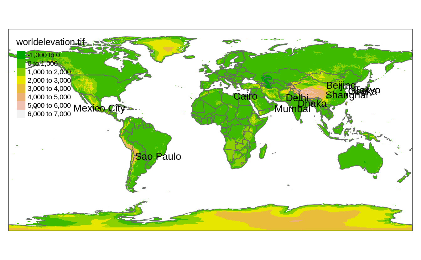
FIGURE 4.1: A map representing three shapes (worldelevation, worldvector, and worldcities) using four layers.
In this example, we use three shapes: worldelevation which is a stars object containing an attribute called "worldelevation.tif", worldvector which is an sf object with country borders, and worldcities, which is an sf object that contains metropolitan areas of at least 20 million inhabitants.
Each tm_shape() function call is succeeded by one or more layer functions.
In the example these are tm_raster(), tm_borders(), tm_dots() and tm_text().
We will describe layer functions in detail in the next chapter.
For this chapter, it is sufficient to know that each layer function call defines how the spatial data specified with tm_shape() is plotted.
Shape objects can be used to plot multiple layers.
In the example, shape worldcities is used for two layers, tm_dots() and tm_text().
4.2 Shapes hierarchy
The order of the tm_shape() functions’ calls is crucial.
The first tm_shape(), known as the main shape, is not only shown below the following shapes, but also sets the projection and extent of the whole map.
In Figure 4.1, the worldelevation object was used as the first shape, and thus the whole map has the projection and extent of this object.
However, we can quickly change the main shape with the is.master argument.
In the following example, we set the worldcities object as the main shape, which limits the output map to the point locations in worldcities (Figure 4.2)7.
tm_shape(worldelevation) +
  tm_raster("worldelevation.tif", palette = terrain.colors(8)) +
tm_shape(worldvector) +
  tm_borders() +
tm_shape(worldcities, is.master = TRUE) +
  tm_dots() +
  tm_text("name")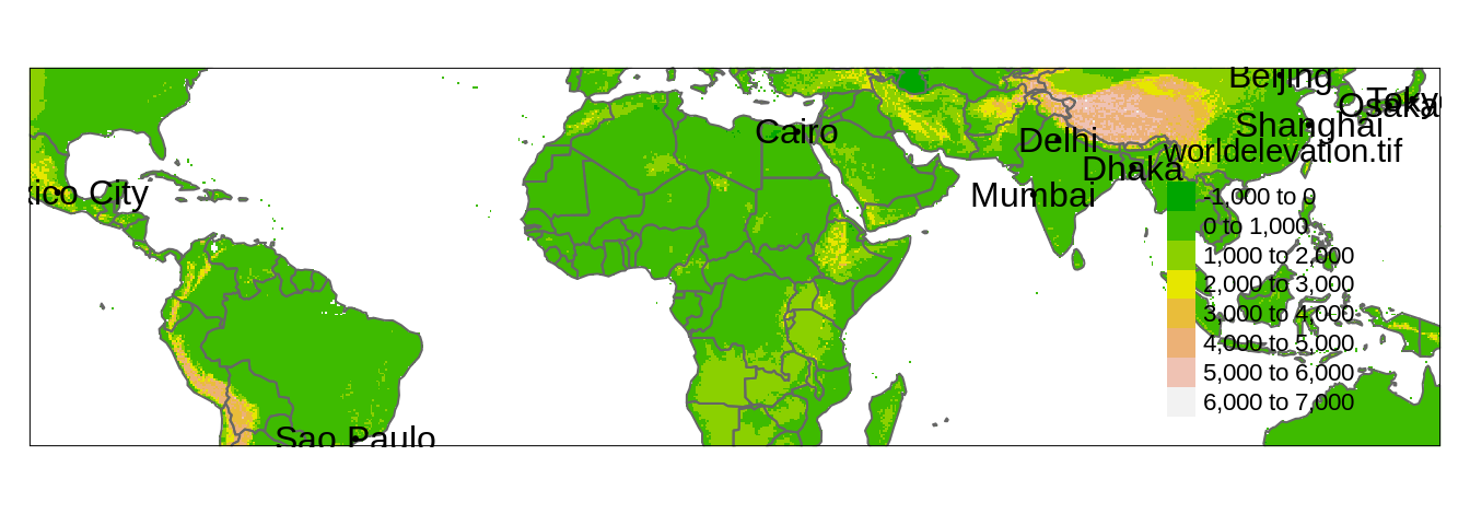
FIGURE 4.2: A map representing three shapes (worldelevation, worldvector, and worldcities) using four layers and zoomed into the locations in the worldcities object.
4.3 Map projection
As we mentioned in the previous section, created maps use the projection from the main shape.
However, we often want to create a map with a different projection, for example to preserve a specific map property (Chapter 2.4).
We can do this in two ways.
The first way to use a different projection on a map is to reproject the main data before plotting, as shown in Section 2.4.6.
The second way is to specify the map projection using the projection argument of tm_shape().
This argument expects either some crs object or a CRS code.
In the next example, we set projection to 8857.
This number represents EPSG 8857 of a projection called Equal Earth (Šavrič, Patterson, and Jenny 2019).
The Equal Earth projection is an equal-area pseudocylindrical projection for world maps similar to the non-equal-area Robinson projection (Figure 2.10).
Reprojections of vector data are usually straightforward because each spatial coordinate is reprojected individually.
However, reprojecting of raster data is more complex and requires using one of two approaches.
The first approach (raster.warp = TRUE) applies raster warping, which is a name for two separate spatial operations: creation of a new regular raster object and computation of new pixel values through resampling (for more details read Chapter 6 of Lovelace, Nowosad, and Muenchow (2019)).
This is the default option in tmap, however, it has some limitations.
Figure 4.3:A shows the world elevation raster reprojected to Equal Earth.
Some of you can quickly noticed that certain areas, such as parts of Antarctica, New Zealand, Alaska, and the Kamchatka Peninsula, are presented twice: with one version being largely distorted.
Another limitation of raster.warp = TRUE is the use of the nearest neighbor resampling only - while it can be a proper method to use for categorical rasters, it can have some unintended consequences for continuous rasters (such as the "worldelevation.tif" data).
tm_shape(worldelevation, projection = 8857) +
  tm_raster("worldelevation.tif", palette = terrain.colors(8))
The second approach (raster.warp = FALSE) computes new coordinates for each raster cell keeping all of the original values and results in a curvilinear grid.
This calculation could deform the shapes of original grid cells, and usually curvilinear grids take a longer time to plot8.
Figure 4.3:B shows an example of the second approach, which gave a better result in this case without any spurious lands. However, creation of the B map takes about ten times longer than the A map.
tm_shape(worldelevation, projection = 8857, raster.warp = FALSE) +
  tm_raster("worldelevation.tif", palette = terrain.colors(8))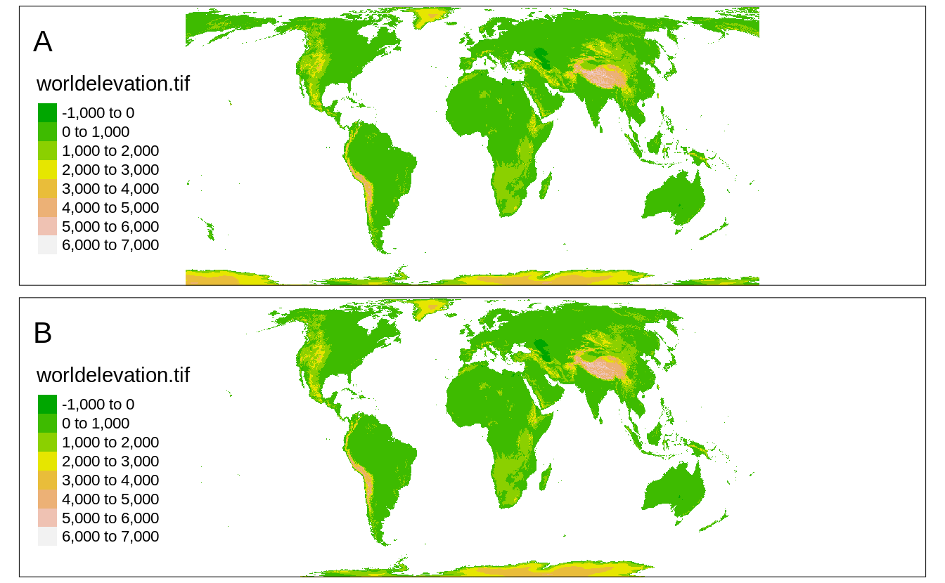
FIGURE 4.3: Two elevation maps in the Equal Earth projection: (A) created using raster.warp = TRUE, (B) created using raster.warp = FALSE.
4.4 Map extent
Another important aspect of mapping, besides projection, is its extent - a portion of the area shown in a map. This is not an issue when the extent of our spatial data is the same as we want to show on a map. However, what should we do when the spatial data contains a larger region than we want to present?
Again, we could take two routes.
The first one is to preprocess our data before mapping - this can be done with vector clipping (e.g., st_intersection()) and raster cropping (e.g., st_crop()).
We would recommend this approach if you plan to work on the smaller data in the other parts of the project.
The second route is to specify the map extent in tmap.
tmap allows specifying map extent using three approaches.
The first one is to specify minimum and maximum coordinates in the x and y directions that we want to represent.
This can be done with a numeric vector of four values in the order of minimum x, minimum y, maximum x, and maximum y, where all of the coordinates need to be specified in the input data units^[This can also be done with the object of class st_bbox or a 2 by 2 matrix.
In the following example, we limit our map extent to the rectangular area between x from -15 to 45 and y from 35 to 65 (Figure 4.4).
tm_shape(worldelevation, bbox = c(-15, 35, 45, 65)) +
  tm_raster("worldelevation.tif", palette = terrain.colors(8))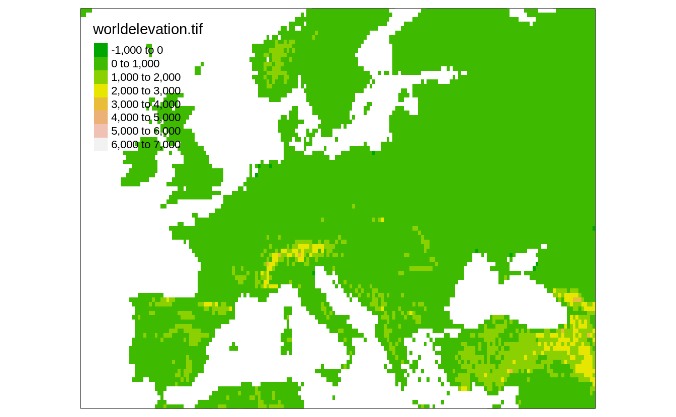
FIGURE 4.4: Global elevation data limited to the extent of the specified minimum and maximum coordinates.
The second approach allows setting the map extent based on a search query.
In the code below, we limit the map extent to the area of "Europe" (Figure 4.5).
This approach uses the OpenStreetMap tool called Nominatim to automatically generate minimum and maximum coordinates in the x and y directions based on the provided query.
tm_shape(worldelevation, bbox = "Europe") +
  tm_raster("worldelevation.tif", palette = terrain.colors(8))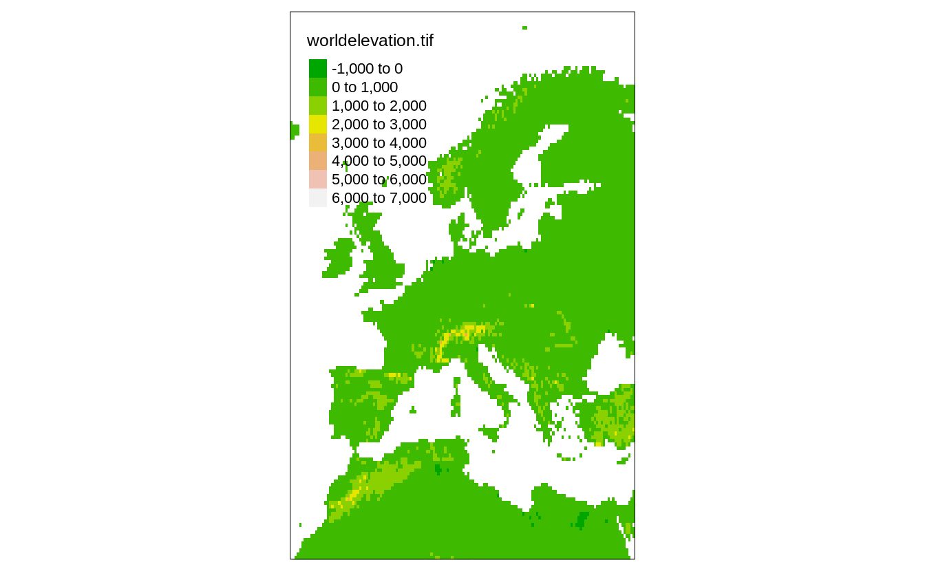
FIGURE 4.5: Global elevation data limited to the extent specified with the ‘Europe’ query.
In the last approach, the map extent is based on another existing spatial object.
Figure 4.6 shows the elevation raster data (worldelevation) limited to the edge coordinates from worldcities.
tm_shape(worldelevation, bbox = worldcities) +
  tm_raster("worldelevation.tif", palette = terrain.colors(8))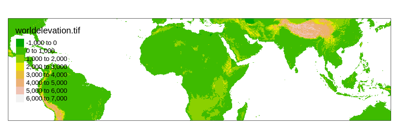
FIGURE 4.6: Global elevation data limited to the extent of the other spatial object.
4.5 Data simplification
Geometries in spatial vector data consists of sets of coordinates (Section 2.2.1).
Spatial vector objects grow larger with more features to present and more details to show, and this also has an impact on time to render a map.
Figure 4.7:A shows a map of countries from the worldvector object.
This level of detail can be good for some maps, but sometimes the number of details can make reading the map harder.
To show a simplified (smoother) version of vector data, we can use the simplify argument of tm_shape()9.
It expects a numeric value from 0 to 1 - a proportion of vertices in the data to retain.
In the example below, we set simplify to 0.05, which keeps 5% of vertices (Figure 4.7:B).
The process of simplification can also be more controlled.
By default, the underlining algorithm (called the Visvalingam method, learn more at https://bost.ocks.org/mike/simplify/), removes small features, such as islands in our case.
This could have far-reaching consequences - in the process of simplification, we could remove some countries!
To prevent the deletion of small features, we also need to set keep.units to TRUE.
Figure 4.7:C shows the result of such an operation.
Now, our map contains all of the countries from the original data, but in a simplified form.
keep.units = TRUE, however, does not keep all of the subfeatures.
In the case of one country consisting of many small polygons, only one is sure to be retained.
For example, look at New Zealand, which is now only represented by Te Waipounamu (the South Island).
To keep all of the spatial geometries (even the smallest of islands), we should also specify keep.subunits to TRUE.
Figure 4.7:D contains a simplified map, where each spatial geometry of the original map still exists, but in a less detailed form.
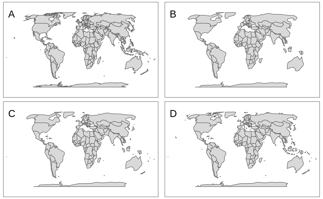
FIGURE 4.7: A map of world’s countries based on: (A) original data, (B) simplified data with 5% of vertices kept, (C) simplified data with 5% of vertices, and all features kept, (D) simplified data with 5% of vertices, all features, and all polygons kept.
All of the about vector simplification functions use the ms_simplify() from the rmapshaper package .
Therefore, you can customize the data simplification even further using other arguments of ms_simplify() (except for the arguments input, keep, keep_shapes, and explode).
Raster data is represented by a grid of cells (Section 2.2.2), and the number of cells impacts the time to render a map.
Rasters with hundreds of cells will be plotted quickly, while rasters with hundreds of millions or billions of cells will take a lot of time (and RAM) to be shown.
Therefore, the tmap package downsamples large rasters by default to be below 10,000,000 cells in the plot mode and 1,000,000 cells in the view mode.
This values can be adjusted with the max.raster argument of tmap_options(), which expects a named vector with two elements - plot and view.
(Figure 4.8:A).
tmap_options(max.raster = c(plot = 5000, view = 2000))
tm_shape(worldelevation) +
  tm_raster("worldelevation.tif")
Raster downsampling can be also disabled with the raster.downsample argument of tm_shape() (Figure 4.8:B).
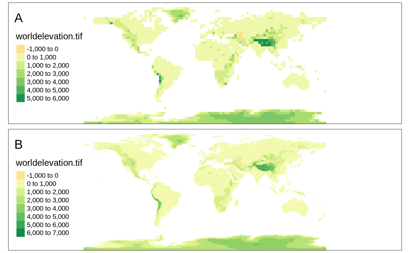
FIGURE 4.8: (A) A raster map with the decreased resolution, (B) a raster map in the original resolution.
Any tmap options can be reset (set to default) with tmap_options_reset() (We explain tmap_options() in details in Chapter 11).
References
Lovelace, R, J Nowosad, and J Muenchow. 2019. Geocomputation with R. Chapman and Hall/CRC Press.
Šavrič, Bojan, Tom Patterson, and Bernhard Jenny. 2019. “The Equal Earth Map Projection.” International Journal of Geographical Information Science 33 (3): 454–65. https://doi.org/10/cs8v.
However, tmap also accepts other spatial objects, e.g., of
sp,raster, andterraclasses.↩︎We will show how to adjust margins and text locations later in the book↩︎
For more details of the first approach see
?stars::st_warp()and of the second approach see?stars::st_transform().↩︎Vector data simplification requires the rmapshaper package to be installed.↩︎