With the tmap package, thematic maps can be generated with great
flexibility. The syntax for creating plots is similar to that of
ggplot2, but tailored to maps. This vignette is for those
who want to get started with tmap within a couple of minutes.
For more context on R’s geographic capabilities we recommend the
online version of the book Geocomputation with R. The Making maps with R chapter of
the book provides many more context and abundant code examples of map
making with tmap and other packages. Other good resources
are the vignettes of the sf
package.
Hello World!
A good place to start is to create a map of the world. After installing tmap, the following lines of code should create the map shown below:
library(tmap)
##
## Attaching package: 'tmap'
## The following object is masked from 'package:datasets':
##
##     rivers

tm_shape(World) +
    tm_polygons("HPI")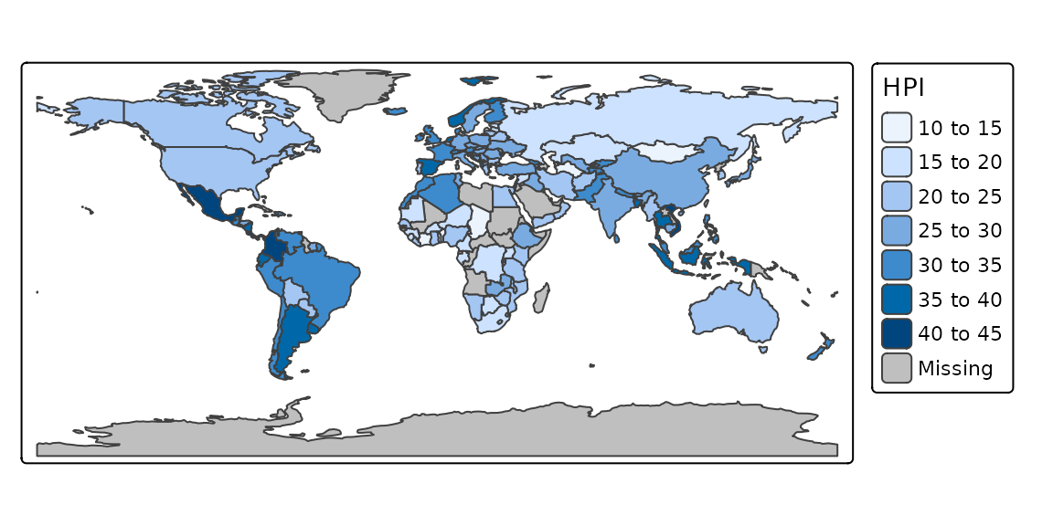
The object World is a spatial object of class
sf from the sf package; it is a
data.frame with a special column that contains a geometry
for each row, in this case polygons. In order to plot it in tmap, you
first need to specify it with tm_shape(). Layers can be
added with the + operator, in this case
tm_polygons(). There are many layer functions in tmap,
which can easily be found in the documentation by their tm_
prefix. See also ?'tmap-element'.
Interactive maps
Each map can be plotted as a static image or viewed interactively
using "plot" and "view" modes, respectively.
The mode can be set with the function tmap_mode, and
toggling between the modes can be done with the ‘switch’
ttm() (which stands for toggle thematic map.
tmap_mode("view")
## ℹ tmap mode set to "view".

tm_shape(World) +
    tm_polygons("HPI")
Multiple shapes and layers
A shape is a spatial object (with a class from sf,
stars, or terra). Multiple shapes and also
multiple layers per shape can be plotted:
tmap_mode("plot")
## ℹ tmap mode set to "plot".
tm_shape(land) +
    tm_raster("elevation", palette = terrain.colors(10)) +
tm_shape(World) +
    tm_borders("white", lwd = .5) +
    tm_text("iso_a3", size = "AREA") +
tm_shape(metro) +
    tm_symbols(col = "red", size = "pop2020", scale = .5) +
tm_legend(show = FALSE)
##
## ── tmap v3 code detected ───────────────────────────────────────────────────────
## [v3->v4] `tm_raster()`: migrate the argument(s) related to the scale of the
## visual variable `col` namely 'palette' (rename to 'values') to col.scale =
## tm_scale(<HERE>).[v3->v4] `symbols()`: use 'fill' for the fill color of polygons/symbols
## (instead of 'col'), and 'col' for the outlines (instead of 'border.col').[v3->v4] `symbols()`: migrate the argument(s) related to the scale of the
## visual variable `size` namely 'scale' (rename to 'values.scale') to size.scale
## = tm_scale_continuous(<HERE>).
## ℹ For small multiples, specify a 'tm_scale_' for each multiple, and put them in
##   a list: 'size.scale = list(<scale1>, <scale2>, ...)'[v3->v4] `tm_legend()`: use 'tm_legend()' inside a layer function, e.g.
## 'tm_polygons(..., fill.legend = tm_legend())'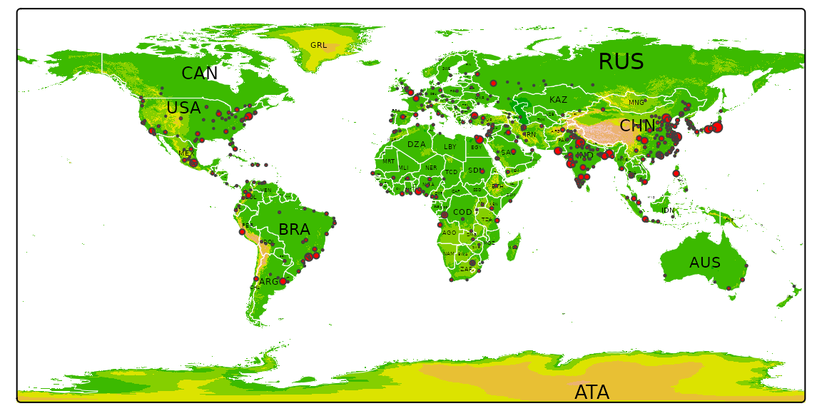
Facets
Facets can be created in three ways:
- By assigning multiple variable names to one aesthetic (in this
example the first argument of
tm_polygons():
tmap_mode("view")
## ℹ tmap mode set to "view".
tm_shape(World) +
    tm_polygons(c("HPI", "economy")) +
tm_facets(sync = TRUE, ncol = 2)- By splitting the spatial data with the
byargument oftm_facets:
tmap_mode("plot")
## ℹ tmap mode set to "plot".

NLD_muni$perc_men <- NLD_muni$pop_men / NLD_muni$population * 100

tm_shape(NLD_muni) +
    tm_polygons("perc_men", palette = "RdYlBu") +
    tm_facets(by = "province")
##
## ── tmap v3 code detected ───────────────────────────────────────────────────────
## [v3->v4] `tm_polygons()`: migrate the argument(s) related to the scale of the
## visual variable `fill` namely 'palette' (rename to 'values') to fill.scale =
## tm_scale(<HERE>).[cols4all] color palettes: use palettes from the R package cols4all. Run 'cols4all::c4a_gui()' to explore them. The old palette name "RdYlBu" is named "rd_yl_bu" (in long format "brewer.rd_yl_bu")
## Multiple palettes called "rd_yl_bu" found: "brewer.rd_yl_bu", "matplotlib.rd_yl_bu". The first one, "brewer.rd_yl_bu", is returned.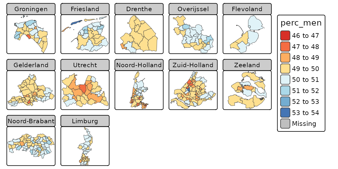
- By using the
tmap_arrangefunction:
tmap_mode("plot")
## ℹ tmap mode set to "plot".

tm1 <- tm_shape(NLD_muni) + tm_polygons("population", convert2density = TRUE)
##
## ── tmap v3 code detected ───────────────────────────────────────────────────────
## [v3->v4] `tm_polygons()` `convert2density` is deprecated.
## ℹ Divide the variable values by the polygon areas manually (obtain the areas
##   with 'sf::st_area()').
tm2 <- tm_shape(NLD_muni) + tm_bubbles(size = "population")

tmap_arrange(tm1, tm2)
## [plot mode] fit legend/component: Some legend items or map compoments do not fit well, and are therefore rescaled. Set the tmap option 'component.autoscale' to FALSE to disable rescaling.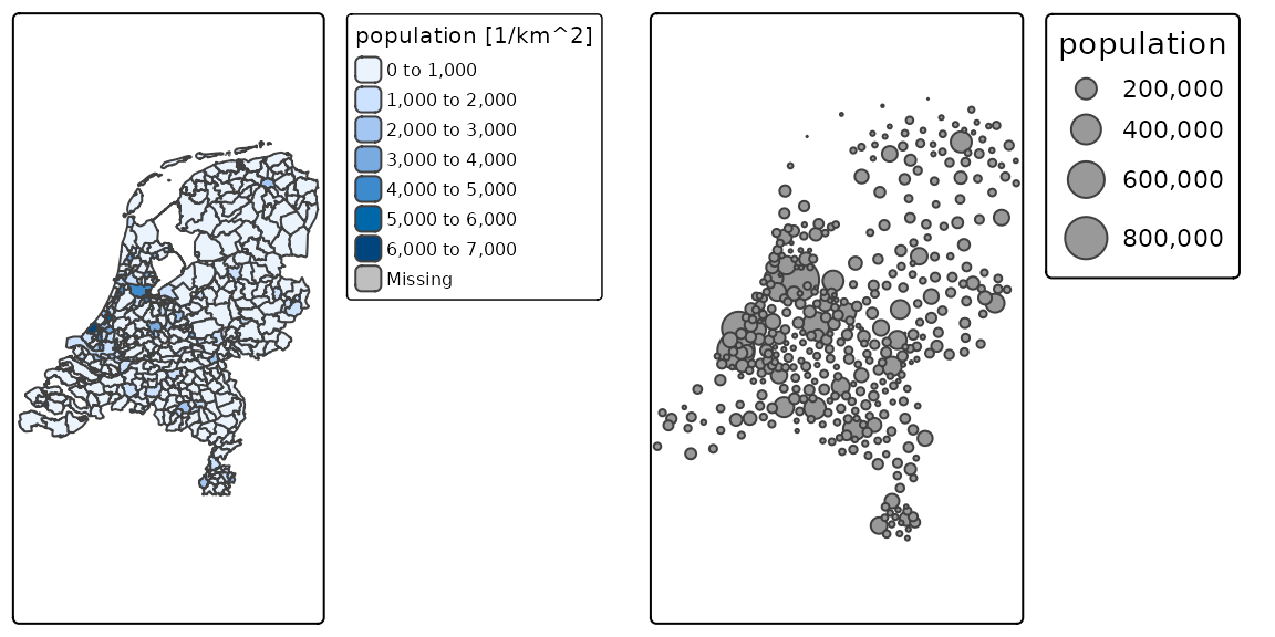
Basemaps and overlay tile maps
Tiled basemaps can be added with the layer function
tm_basemap. Semi-transparent overlay maps (for example
annotation labels) can be added with tm_tiles.
tmap_mode("view")
## ℹ tmap mode set to "view".
tm_basemap("Stamen.Watercolor") +
tm_shape(metro) + tm_bubbles(size = "pop2020", col = "red") +
tm_tiles("Stamen.TonerLabels")
See a preview
of the available tilemaps. This list is also accessible in R:
leaflet::providers.
Options and styles
The functions tm_layout() and tm_view() are
used to specify the map layout and the interactive aspects respectively.
These functions can be used in the same way as the layer functions,
e.g.
tmap_mode("plot")
## ℹ tmap mode set to "plot".

tm_shape(World) +
    tm_polygons("HPI") +
tm_layout(bg.color = "skyblue", inner.margins = c(0, .02, .02, .02))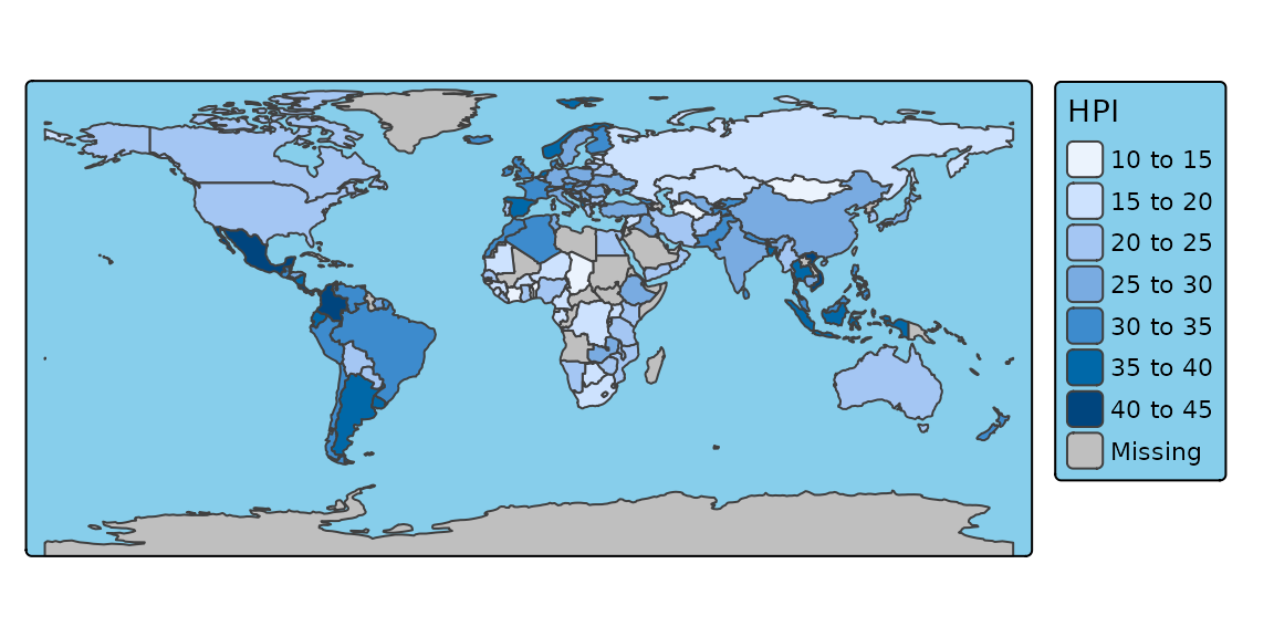
These options, as well as a couple of others, can also be set within
with tmap_options, which works in the same way as the base
R function options. The main advantage is that these
options are set globally, so they do not have to be specified in each
map, for the duration of the session.
tmap_options(bg.color = "black", legend.text.color = "white")

tm_shape(World) +
    tm_polygons("HPI", legend.title = "Happy Planet Index")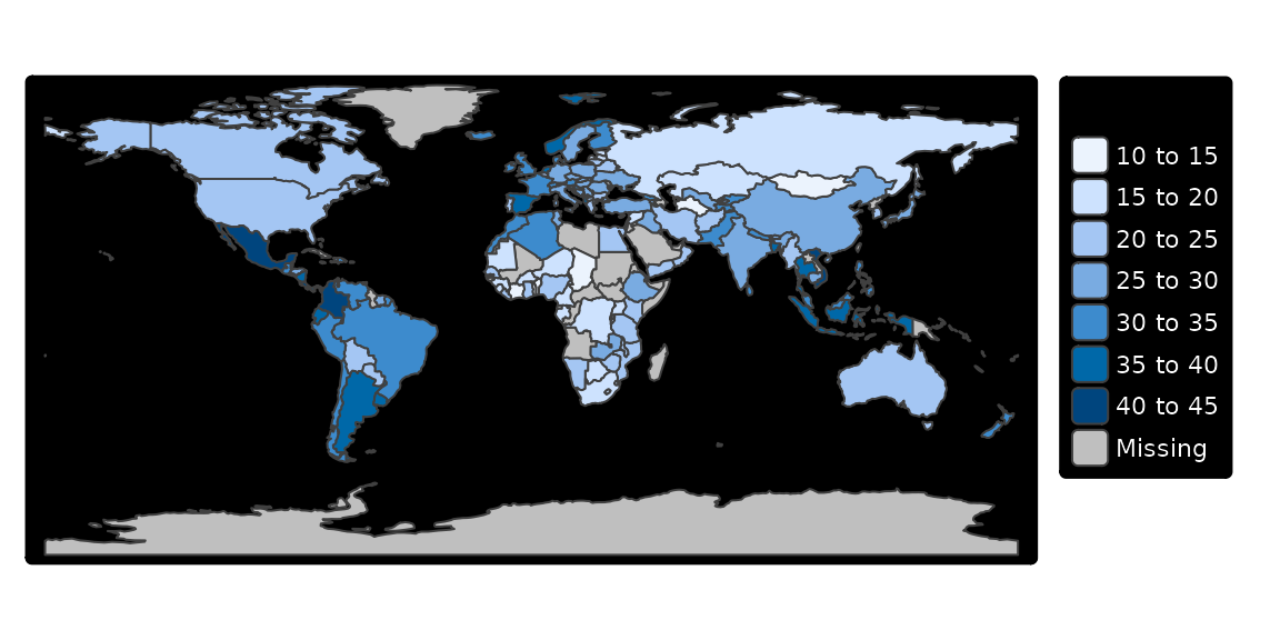
A style is a certain configuration of the tmap options.
tmap_style("classic")
## style set to "classic"
## other available styles are: "white" (tmap default), "gray", "natural", "cobalt", "albatross", "beaver", "bw", "watercolor"
## tmap v3 styles: "v3" (tmap v3 default), "gray_v3", "natural_v3", "cobalt_v3", "albatross_v3", "beaver_v3", "bw_v3", "classic_v3", "watercolor_v3"

tm_shape(World) +
    tm_polygons("HPI", legend.title = "Happy Planet Index")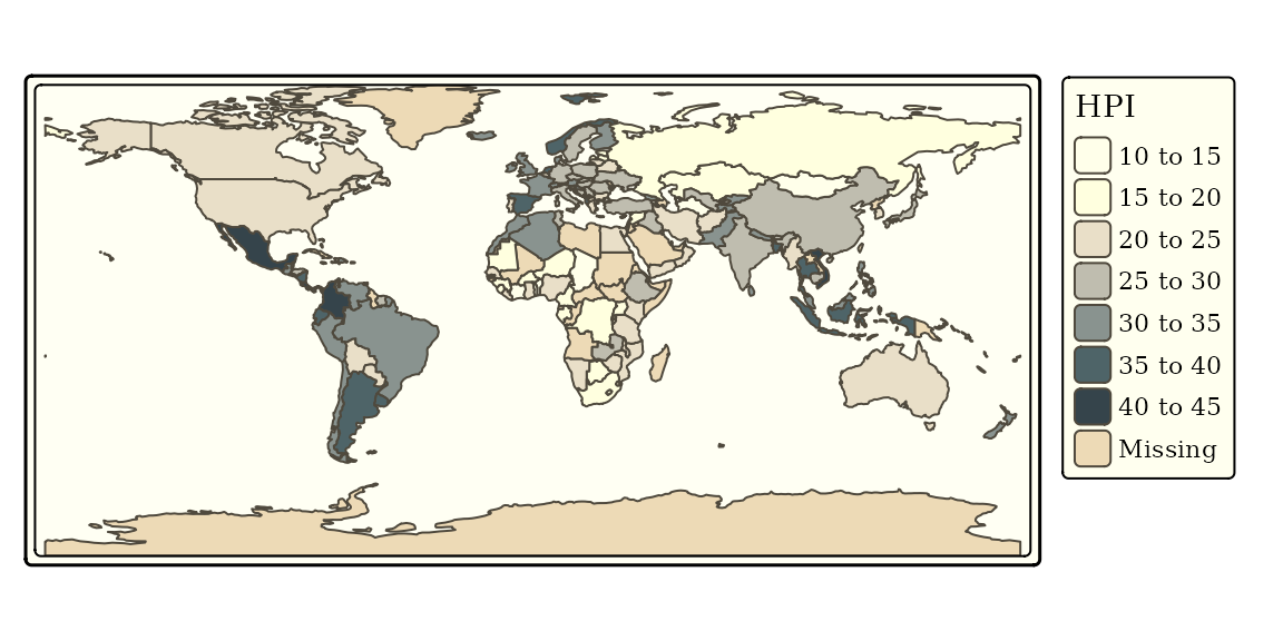
# see what options have been changed
tmap_options_diff()
## current tmap options (style "classic") that are different from default tmap options (style "white"):
## $frame.double.line
## [1] TRUE
##
## $color.sepia.intensity
## [1] 0.7
##
## $text.fontfamily
## [1] "serif"
##
## $compass.type
## [1] "rose"

# reset the options to the default values
tmap_options_reset()
## tmap options successfully reset
New styles can be created; see ?tmap_options.
Exporting maps
tm <- tm_shape(World) +
    tm_polygons("HPI", legend.title = "Happy Planet Index")

tm
ttmp()
## ℹ tmap mode set to "view".Shiny integration
It is possible to use tmap in shiny:
# in UI part:
tmapOutput("my_tmap")

# in server part
output$my_tmap = renderTmap({
    tm_shape(World) + tm_polygons("HPI", legend.title = "Happy Planet Index")
})
See ?renderTmap for a working example.
Quick thematic map
Maps can also be made with one function call. This function is
qtm:
qtm(World, fill = "HPI", fill.palette = "RdYlGn")
##
## ── tmap v3 code detected ───────────────────────────────────────────────────────
## [v3->v4] `qtm()`: migrate the argument(s) related to the scale of the visual
## variable `fill` namely 'palette' (rename to 'values') to fill.scale =
## tm_scale(<HERE>).