The next major update of tmap will be a massive one. Although tmap is well-known and widely used in the R spatial community, there are a couple of bottlenecks that make it difficult to maintain and extend. The upcoming tmap version 4 (tmap v4) aims to overcome these shortcomings. This document provides an overview of the new features and improvements that will be available in tmap v4.
Extendability
First and foremost, tmap v4 will be fully extendable. More precisely, the following aspects can be extended:
Map layers: we are not limited anymore by the fixed set of
tm_polygons(),tm_lines(),tm_symbols(), andtm_raster()(and their derivatives such astm_borders()andtm_dots()), but any layer of interest can be developed as an extension of tmap. We will illustrate this later withtm_cartogram().Visual variables: there will be many more visual variables (e.g.,
fillorcol) available. We will illustrate this in the next section, where we already implemented five new visual variables fortm_polygons(). Moreover, it will be much easier for developers to add new visual variables to map layer functions.Graphics engine: tmap contains two modes,
plotandview(which are based on grid graphics and leaflet respectively) but the framework makes it possible to add other modes as well.Spatial data classes: tmap is build on sf and stars, and supports terra objects natively. Moreover, for developers, it will be easier to incorporate other classes as well.
Visual variables
As mentioned before, we have added more visual variables, and it will be easier for developers to add new visual variables. Moreover, we have reordered the arguments that specify and configure the visual variables.
The arguments that specify visual variables themselves will remain the same.
For example, the main aesthetic in tm_polygons() is fill, which defines the fill color of the polygons.
However, other arguments of the layer functions are organized differently.
Thus, each aesthetic will only have five arguments:
- the visual variable itself (
fill) - the scale (
fill.scale) - the legend (
fill.legend) - the chart (
fill.chart) - an argument that decides whether scales are applied freely across facets (
fill.free)
The scales and legends are discussed in the next sections.
Below you can see a basic comparison of the tmap version 3 and 4 syntax:
# tmap v3
tm_shape(World) +
    tm_polygons(fill = "HPI",
                palette = "PRGn",
                title = "Happy Planet Index")
# tmap v4
tm_shape(World) +
    tm_polygons(fill = "HPI",
                fill.scale = tm_scale_intervals(values = "purple_green"),
                fill.legend = tm_legend(title = "Happy Planet Index"))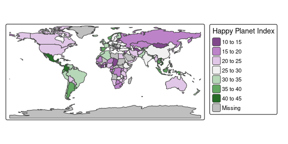
In tmap v4, tm_polygons() will have the visual variables of fill, col, fill_alpha, col_alpha, lwd, lty, and eventually also pattern.
The other standard map layers will also have additional visual variables.
A data variable can be mapped to each of them, using different scales (see next section for an overview).
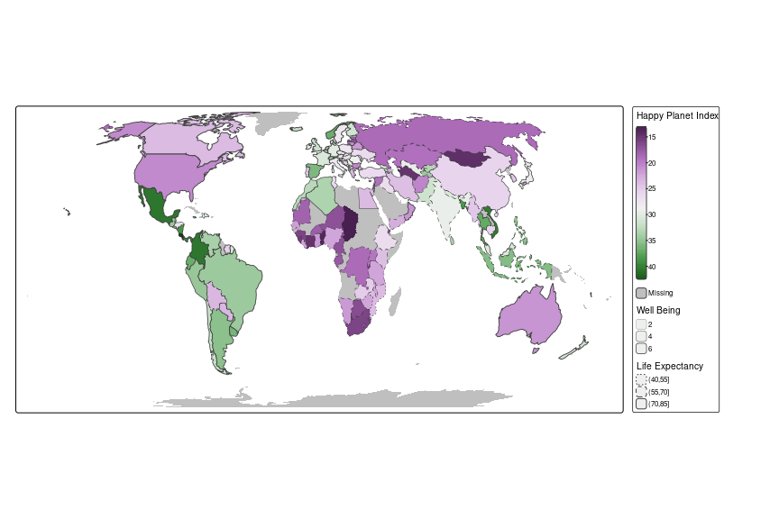
The next example uses fill, lwd (line width), and lty (line type) as visual variables, which was not possible in tmap v3:
# tmap v3
# ... not possible :(
# tmap v4
World$life_exp_class = cut(World$life_exp, breaks = seq(40, 85, by = 15))

tm_shape(World, crs = "+proj=eck4") +
    tm_polygons(fill = "HPI",
                fill.scale = tm_scale_continuous(values = "purple_green"),
                fill.legend = tm_legend(title = "Happy Planet Index"),
                lwd = "well_being",
                lwd.scale = tm_scale_continuous(value.neutral = 1,
                                                values = c(0, 5),
                                                label.na = ""),
                lwd.legend = tm_legend(title = "Well Being"),
                lty = "life_exp_class",
                lty.scale = tm_scale_ordinal(values = c("dotted", "dashed", "solid"),
                                             value.na = "blank",
                                             value.neutral = "solid",
                                             label.na = ""),
                lty.legend = tm_legend(title = "Life Expectancy")
    )
Besides these visual mapping visual variables, which map data variables to visual variables, there is also another group of visual variables, namely (data-driven) transformation visual variables. They are used to transform spatial objects. We call it data-driven, because content data are used as input for this spatial transformation. An example is the cartogram, which will be shown in the next section. Using the cartogram method, the polygons are distorted such that their sizes are (approximately) proportional to a data variable.
Map layers (e.g. cartogram)
It will be easy for developers to add new map layers as extension.
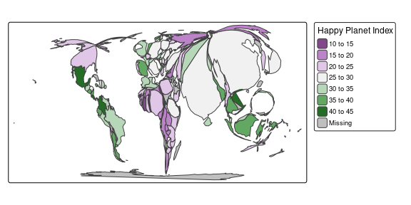
We illustrate this by a new map layer, tm_cartogram().
Cartograms could already be made with tmap v3, but it explicitly required transforming the data using the cartogram package before mapping.
# tmap v3
library(cartogram)
World_carto = World |>
  sf::st_transform(World, crs = "+proj=eck4") |>
  cartogram_cont(weight = "pop_est")

tm_shape(World_carto, crs = "+proj=eck4") +
  tm_polygons(fill = "HPI",
              palette = "PRGn",
              title = "Happy Planet Index")
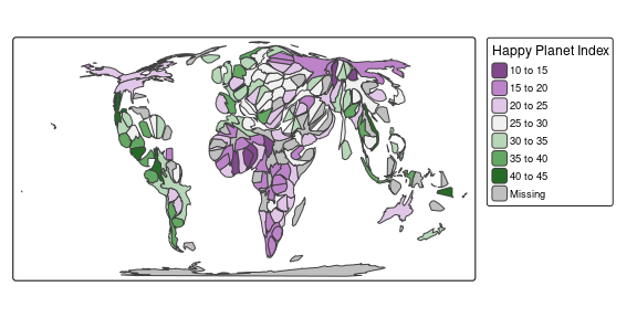
In tmap v4, there will be a direct function tm_cartogram() (using the cartogram package under the hood), which uses the transformation aesthetic size and inherits all visual variables from tm_polygons():
# tmap v4
if (requireNamespace("cartogram")) {
tm_shape(World, crs = "+proj=eck4") +
    tm_cartogram(size = "pop_est",
                 fill = "HPI",
                 fill.scale = tm_scale_intervals(values = "purple_green"),
                 fill.legend = tm_legend(title = "Happy Planet Index")) +
    tm_place_legends_right(width = 0.2)
}
A benefit of having cartograms directly in tmap is that it makes possible to use the available scaling functions. For example, to achieve a more “balanced” cartogram, we can apply a logarithmic transformation (base 10):
# tmap v3
library(cartogram)
World_carto = World |>
  sf::st_transform(World, crs = "+proj=eck4") |>
  dplyr::mutate(pop_est_log10 = log10(pop_est)) |>
  cartogram_cont(weight = "pop_est_log10")

tm_shape(World_carto) +
  tm_polygons(fill = "HPI",
              palette = "PRGn",
              title = "Happy Planet Index")
# tmap v4
if (requireNamespace("cartogram")) {
tm_shape(World, crs = "+proj=eck4") +
    tm_cartogram(size = "pop_est",
                 size.scale = tm_scale_continuous_log1p(),
                 fill = "HPI",
                 fill.scale = tm_scale_intervals(values = "purple_green"),
                 fill.legend = tm_legend(title = "Happy Planet Index")) +
    tm_place_legends_right(width = 0.2)
}
Scales
Scales are used to map data variables to visual variables. Scales are not new in tmap v4, but now they are used more explicitly.
The following table shows the currently available scales:
| Scale | Main Data Type | Example |
|---|---|---|
tm_scale_categorical() |
categorical (factor) |
Fruit type |
tm_scale_ordinal() |
categorical (ordered) |
Education level |
tm_scale_intervals() |
numerical (integer or numeric) |
Age group |
tm_scale_continuous() |
numerical (numeric) |
Height |
tm_scale_log10() |
numerical (numeric) |
Income |
tm_scale_discrete() |
numerical (integer) |
Number of children |
The main data type (second column) is the data type for which the scale is supposed to be applied.
Any scale can be applied to any data type (even though it might not make sense), with one exception: continuous (and log10) scales cannot be applied to visual variables that can only take a finite set of values, for example shapes of a symbol or types of lines.
By default, tm_scale_categorical(), tm_scale_ordinal(), and tm_scale_intervals() are used for data of class factor, ordered and numeric respectively.
Scales for date/time variables will be included as well.
The main argument of each scale function is values, which are the values for the visual variables.
The following table shows which type of values are required for which visual variable:
| Visual variable | Type of values |
|---|---|
fill and col
|
Color palette |
size and lwd
|
(Exponential) value range |
lty |
Line type, e.g. "dashed"
|
shape |
Shapes (similar to tmap v3) |
fill_alpha and col_alpha
|
Value range |
The default values depend not only on the visual variable, but also on the scale and on whether data values are diverging.
For instance, if tm_scale_intervals() is applied to a numeric variable with both negative and positive values where the visual variable is fill, then a diverging color palette is used.
The following map illustrates what happens when the six scale functions are applied to the same data variable. We use the variable life expectancy (which we round in order to make sure the number of unique values is limited):
Scales existed in tmap v3, but they were applied implicitly via several arguments:
# tmap v3
tm_shape(Africa) +
    tm_polygons(rep("life_exp", 5), style = c("cat", "cat", "pretty", "cont", "log10"),
                palette = list("Set2", "YlOrBr", "YlOrBr", "YlOrBr", "YlOrBr"),
                title = "") +
    tm_layout(panel.labels = c("categorical scale", "ordinal scale", "intervals scale",
                               "continuous scale", "log10 scale"),
              inner.margins = c(0.05, 0.2, 0.1, 0.05),
              legend.text.size = 0.5)

# discrete scale is not possible directly, but only via interval breaks:
tm_shape(Africa) +
    tm_polygons("life_exp", style = "fixed",
                palette = "YlOrBr",
                breaks = 49:76,
                as.count = TRUE,
                title = "") +
    tm_layout(panel.labels = "discrete scale",
              inner.margins = c(0.05, 0.2, 0.1, 0.05),
              legend.text.size = 0.5)
# tmap v4
tm_shape(Africa) +
    tm_polygons(rep("life_exp", 6),
                fill.scale = list(tm_scale_categorical(), tm_scale_ordinal(),
                                  tm_scale_intervals(), tm_scale_continuous(),
                                  tm_scale_continuous_log(), tm_scale_discrete()),
                fill.legend = tm_legend(title = "", position = tm_pos_in("left", "top"))) +
    tm_layout(panel.labels = c("tm_scale_categorical", "tm_scale_ordinal",
                               "tm_scale_intervals", "tm_scale_continuous",
                               "tm_scale_continuous_log", "tm_scale_discrete"),
              inner.margins = c(0.05, 0.2, 0.1, 0.05),
              legend.text.size = 0.5)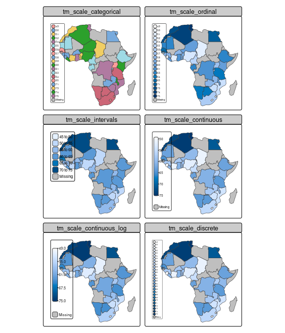
Multivariate scales
It will be possible to assign multiple variables for one aesthetic.
This can be done with the function tm_mv() (which stands for multivariate).
An example is the bivariate choropleth, which is not yet implemented, but will definitely be.
# tmap v3
# ... not possible :(
# tmap v4
tm_shape(World) +
  tm_polygons(
    fill = tm_vars(c("well_being", "footprint"), multivariate = TRUE),
    fill.scale = tm_scale_bivariate(scale1 =  tm_scale_intervals(breaks = c(2, 5, 6, 8)),
                                    scale2 = tm_scale_intervals(breaks = c(0, 3, 6, 20)),
                                    values = "brewer.qualseq")
    )
#> Warning: Values have found that are higher than the highest break. They are
#> assigned to the highest interval
#> Labels abbreviated by the first letters, e.g.: "0 to 3" => "0"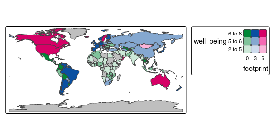
Legends
As you may have noticed in the previous examples, the legends look a bit differently by default.
Positioning
Legends are currently placed outside the map by default in tmap v4. Why? Simply because there is often more space than inside the map.
You might also have noticed that the position of the legends in your maps may be different to the examples here. This is because the placement of the legend depends on the aspect ratio of the device and the map. tmap chooses the position that maximizes the map size. For example, if the map can be bigger with this arrangement, it will place the legend underneath rather than on the right hand side.
Additionally, it is npw possible to place legends in different positions on the map:
# tmap v3
# ... not possible :(
# tmap v4
tm_shape(World) +
  tm_symbols(fill = "HPI",
             size = "pop_est",
             shape = "income_grp",
             size.scale = tm_scale(value.neutral = 0.5),
             fill.legend = tm_legend("Happy Planet Index", position = tm_pos_in("left", "top")),
             size.legend = tm_legend("Population", position = tm_pos_out("left", "center")),
             shape.legend = tm_legend("Income Group", position = tm_pos_out("center", "bottom")))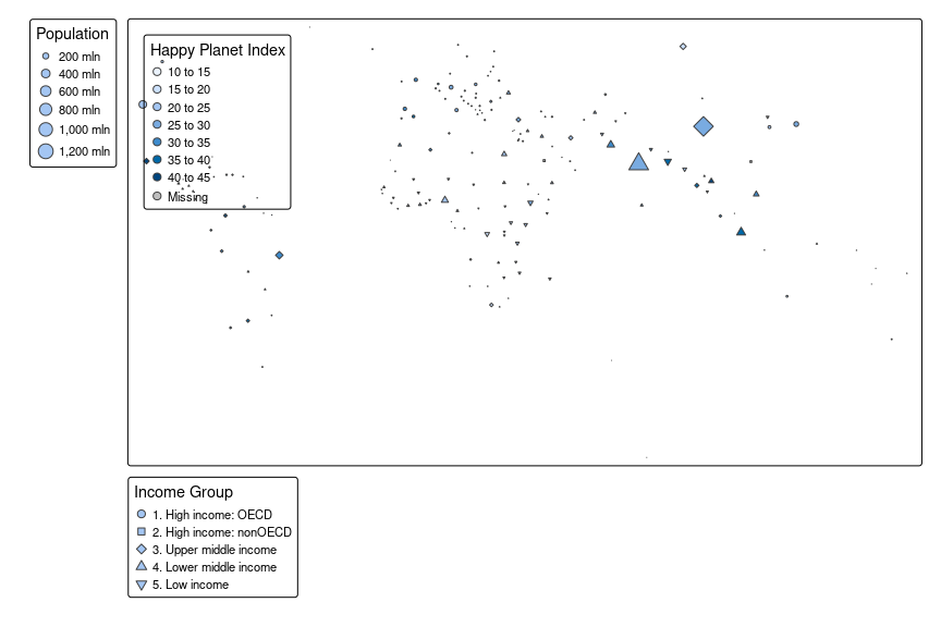
tmap v3 contains many (often complicated) options for rather simple things.
These options are set globally via tmap_options() or within a single plot with tm_layout().
In tmap v4, the options directly related to the layout are accessible via tm_layout().
However, to ease its use, there will be a bunch of handy shortcut functions, such as tm_place_legends_left():
# tmap v3
tm_shape(World) +
    tm_symbols(fill = "HPI",
               size = "pop_est",
               shape = "income_grp") +
    tm_layout(legend.outside.position = "left", legend.outside.size = 0.2)
# tmap v4
tm_shape(World) +
    tm_symbols(fill = "HPI",
               size = "pop_est",
               shape = "income_grp",
               size.scale = tm_scale(value.neutral = 0.5)) +
    tm_place_legends_left(0.2)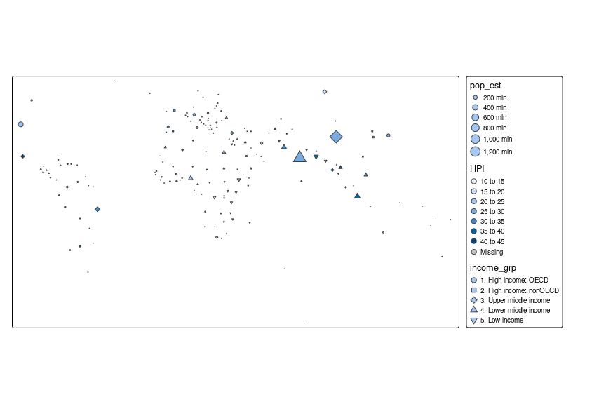
Combined legends
Another new feature is the possibility to combine legends directly, which was quite a hassle in tmap v3.
# tmap v3
tm_shape(metro) +
    tm_symbols(col = "pop2020",
           n = 4,
           size = "pop2020",
           legend.size.show = FALSE,
           legend.col.show = FALSE) +
tm_add_legend("symbol",
              col = RColorBrewer::brewer.pal(4, "YlOrRd"),
              border.col = "grey40",
              size = ((c(10, 20, 30, 40) * 1e6) / 40e6) ^ 0.5 * 2,
              labels = c("0 mln to 10 mln", "10 mln to 20 mln", "20 mln to 30 mln", "30 mln to 40 mln"),
              title = "Population in 2020") +
    tm_layout(legend.outside = TRUE, legend.outside.position = "bottom")
# tmap v4
tm_shape(metro) +
    tm_symbols(fill = "pop2020",
               fill.legend = tm_legend("Population in 2020"),
               size = "pop2020",
               size.scale = tm_scale_intervals(),
               size.legend = tm_legend_combine("fill"))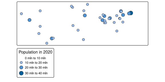
Facets
In tmap v4, there are convenient wrappers tm_facet_wrap() and tm_facet_grid(), where the former wraps the facets, and the latter places the facets in a grid layout.
Furthermore, each visual variable has a free argument, which determines whether scales are free (TRUE) or shared (FALSE) across facets.
In tmap v3 this free argument could be set via tm_facets(), whereas in tmap v4 this argument has been moved to the layer functions:
# tmap v3
tm_shape(World, crs = "+proj=robin") +
    tm_borders() +
tm_shape(World) +
    tm_polygons("life_exp") +
tm_facets("continent", nrow = 3, free.scales.fill = FALSE, free.coords = FALSE)
# tmap v4
tm_shape(World, crs = "+proj=robin") +
    tm_borders() +
tm_shape(World) +
    tm_polygons("life_exp", fill.free = FALSE) +
tm_facets_wrap("continent")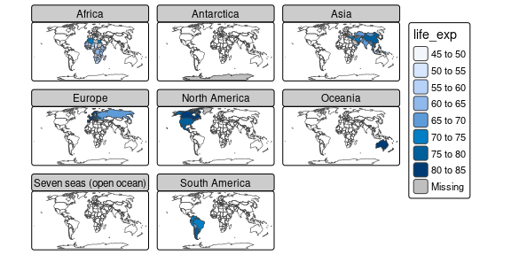
# tmap v3
tm_shape(World, crs = "+proj=robin") +
    tm_borders() +
tm_shape(World) +
    tm_polygons("life_exp") +
tm_facets("continent", nrow = 1, free.scales.fill = TRUE, free.coords = FALSE)
tm_shape(World, crs = "+proj=robin") +
    tm_borders() +
tm_shape(World) +
    tm_polygons("life_exp", fill.free = TRUE) +
tm_facets_stack("continent")
#> Variable(s) "fill" only contains NAs. Legend disabled for tm_scale_intervals, unless breaks are specified
#> Variable(s) "fill" only contains NAs. Legend disabled for tm_scale_intervals, unless breaks are specified
#> [plot mode] fit legend/component: Some legend items or map compoments do not
#> fit well, and are therefore rescaled.
#> ℹ Set the tmap option `component.autoscale = FALSE` to disable rescaling.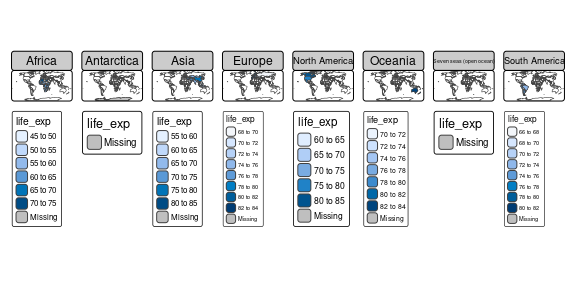
New in tmap v4 is that for facet grid, the free argument can be specified differently for rows and columns, as we will show in the next example:
# tmap v3
# ... not possible :(
# tmap v4
tm_shape(World, crs = "+proj=robin") +
    tm_borders() +
tm_shape(World) +
    tm_polygons(fill = "life_exp",
                fill.scale = tm_scale_intervals(values = "brewer.greens"),
                fill.free = c(rows = FALSE, columns = TRUE)) +
    tm_symbols(size = "gdp_cap_est",
               size.free = c(rows = TRUE, columns = FALSE),
               fill = "red") +
tm_facets_grid("income_grp", "economy") +
tm_layout(meta.margins = c(.2, 0, 0,.1))
#> [plot mode] fit legend/component: Some legend items or map compoments do not
#> fit well, and are therefore rescaled.
#> ℹ Set the tmap option `component.autoscale = FALSE` to disable rescaling.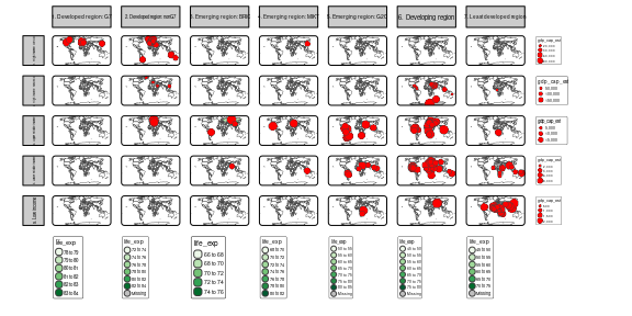
What you see in the map is that life expectancy is shown as polygon fill in green, and GDP per capita as red bubbles. The maps are grouped by income group (rows) and economy (columns). The scale for life expectancy is set to free for the columns. This means that the scale will be applied for each column separately, with a legend per column. The scale for GDP per capita is applied separately for each row.
Graphic engines (modes)
Just like tmap v3, there will be a "plot" and a "view" mode.
However, the framework used in tmap v4 also facilitates developers to write plotting methods for other modes.
For instance, CesiumJS is a great JavaScript library for 3d globe visualizations. It would be awesome to include this in R. When there is a low-level interface between CesiumJS and R (similar to the R package leaflet being an interface between the JS library leaflet and R), it will be relatively easy for developers to add a new mode for these 3d visualizations in tmap v4.
Backward compatibility
In this early development stage, tmap v3 code will not work with tmap v4.
However, when tmap v4 is stable, it will be backward compatible.
Layer function arguments that are no longer used, such as breaks and palette will be deprecated, and internally redirected to the new scale functions.
Furthermore, some of the options will have other options in tmap v4. For instance, legends will be placed outside of the maps by default, and there will be a small space between legend items as shown above.
In order to keep the layout as close as possible to tmap v3, there will be a style that set the options back to the settings used by default in tmap v3.
This can be set with just one command: tmap_style("tmap_v3")
Suggestions
Do you have any suggestions? Please let us know via https://github.com/r-tmap/tmap/issues!
