About the data
A spatial data object contained in tmap is called World. It is a data frame with a row for each country. The columns are the following data variables plus an additional geometry column which contains the geometries (see sf package):
names(World)
#>  [1] "iso_a3"       "name"         "sovereignt"   "continent"    "area"
#>  [6] "pop_est"      "pop_est_dens" "economy"      "income_grp"   "gdp_cap_est"
#> [11] "life_exp"     "well_being"   "footprint"    "HPI"          "inequality"
#> [16] "gender"       "press"        "geometry"
We specify this object with tm_shape (see other vignette) and for convenience assign it to s:
s = tm_shape(World, crs = "+proj=eqearth")Scales: numeric data (intervals)
Each map variable, e.g. fill in tm_polygons can represent a data variable:
s + tm_polygons(fill = "HPI")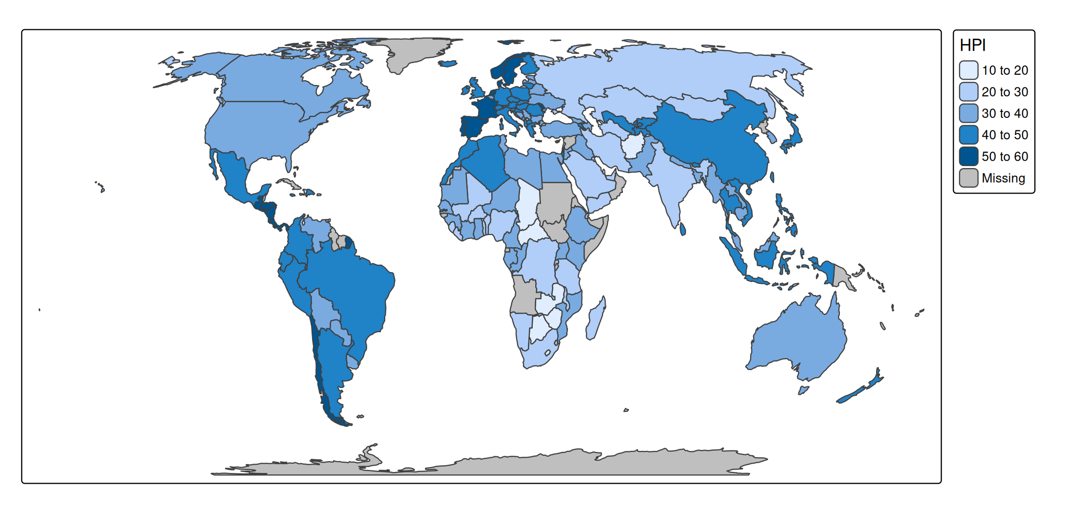
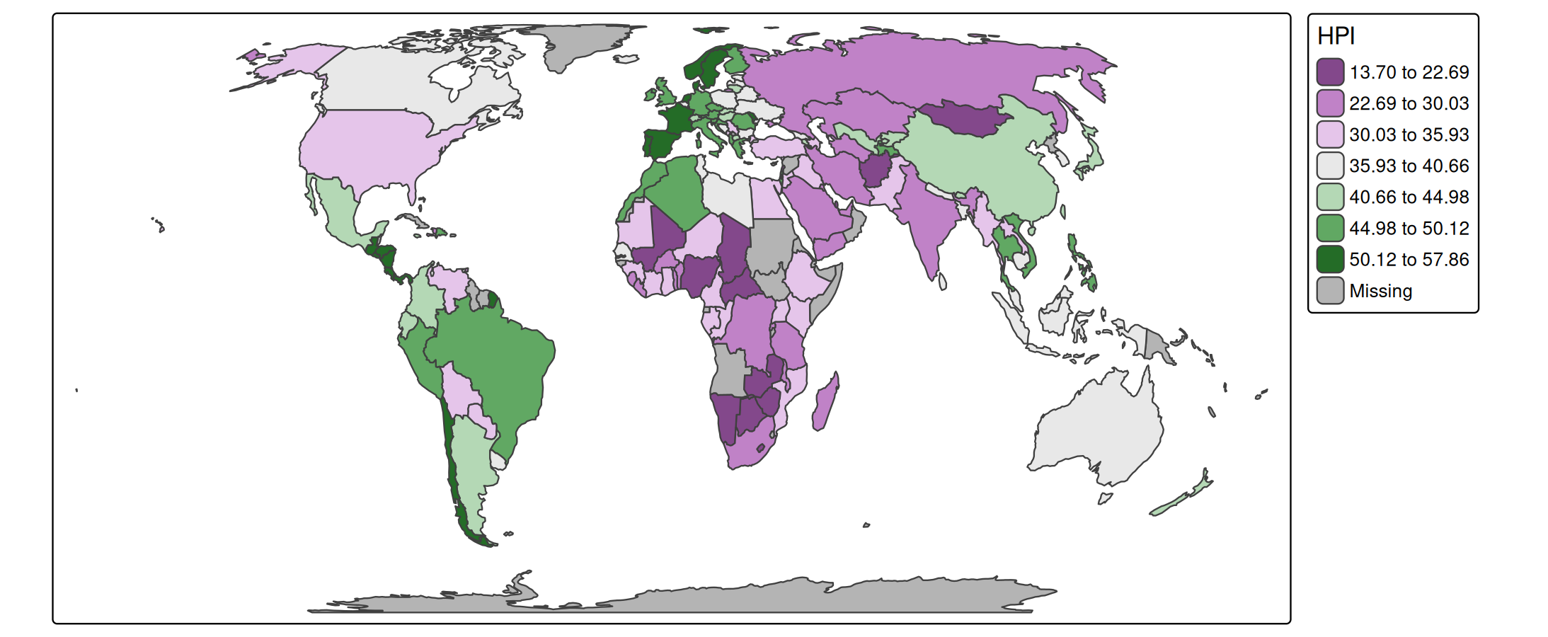
A scale defines how to map the data values to visual values. Numeric data variables (e.g. "HPI" which stands for Happy Planet Index) are by default mapped with a class interval scale to the polygon fill. This can be set explicitly with tm_scale_intervals, via which the intervals can be specified, as well as the visual values (in this case polygon fill colors):
s + tm_polygons(
  fill = "HPI",
  fill.scale = tm_scale_intervals(
    style = "fisher",      # a method to specify the classes
    n = 7,                 # number of classes
    midpoint = 38,         # data value mapped to the middle palette color
    values = "pu_gn_div"   # color palette;
                           # run cols4all::c4a_gui() to explore color palettes
  ))
The style parameter within tm_scale_intervals has a variety of options, including:
fixedsdequalprettyquantilefisherjenks
To specify the classification breaks manually, use style = "fixed" and specify the breaks using breaks = c(0,10,20,30,40,50,60):
s + tm_polygons(
  fill = "HPI",
  fill.scale = tm_scale_intervals(
    n = 6, # for n classes
    style = "fixed",
    breaks = c(0,10,20,30,40,50,60), # you need n+1 number of breaks
    values = "pu_gn_div"
  ))
By default the legend will show bins. Alternatively, the breaks can be printed between the colors:
s + tm_polygons(
  fill = "HPI",
  fill.scale = tm_scale_intervals(
    n = 6,
    style = "fixed",
    breaks = c(0,10,20,30,40,50,60),
    values = "pu_gn_div",
    label.style = "continuous"
  ))
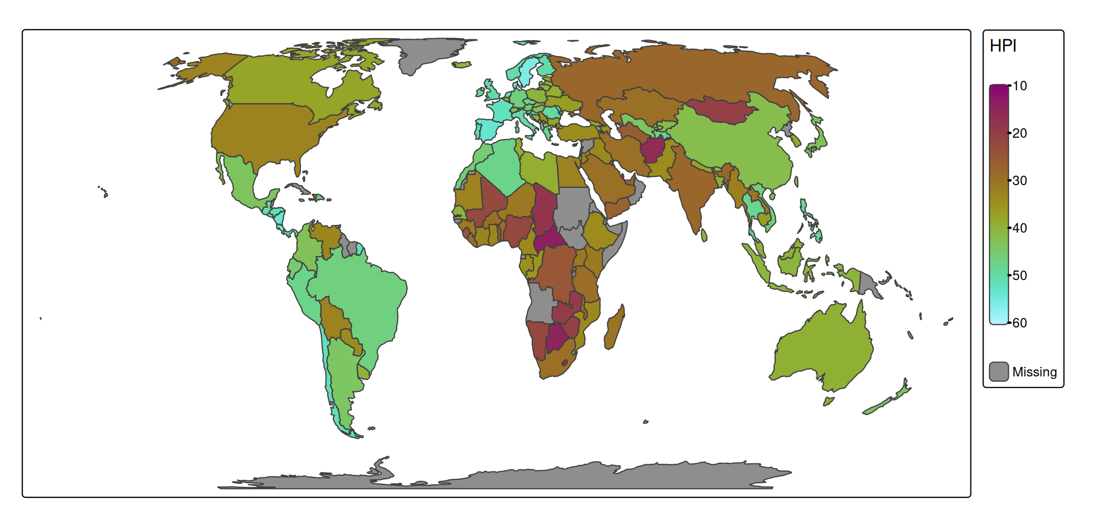
Scales: numeric data (continuous)
An alternative for numeric data variables is the continuous scale:
s +
  tm_polygons(
    fill = "HPI",
    fill.scale = tm_scale_continuous(
      limits = c(10, 60),
      values = "scico.hawaii"))
By default, the limit (so the value range that is mapped to a color gradient) is taken from the actual data value range range(World$HPI, na.rm = T)), which is 13.6980838, 57.8611615. In this example rounded numbers 10 and 60 are specified here. If needed, the position of ticks can be specified via the argument ticks.
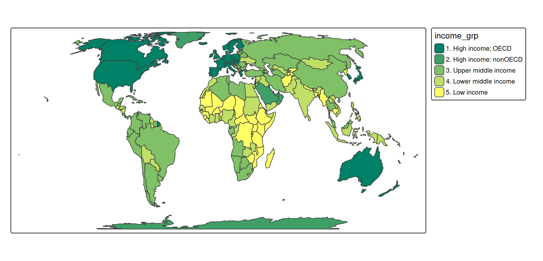
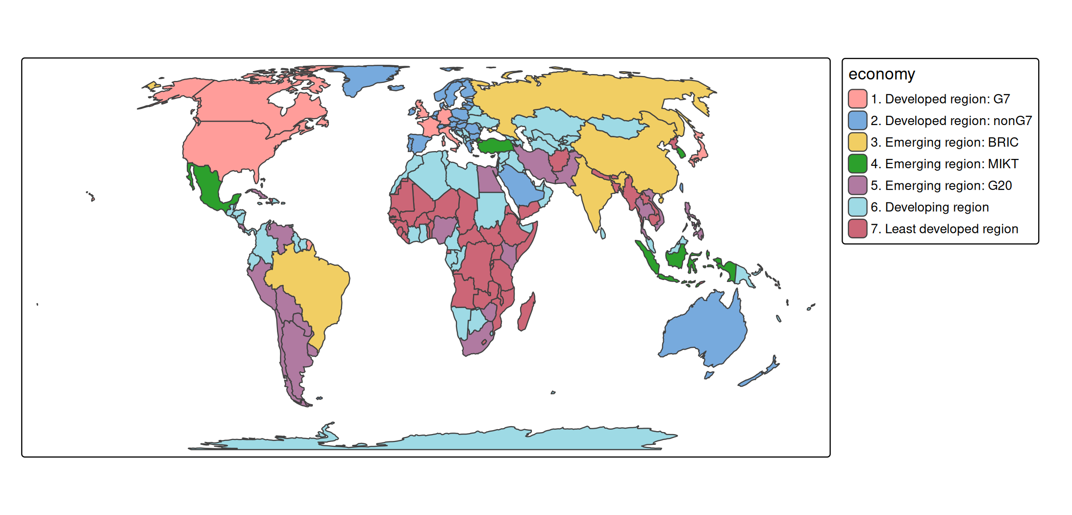
Scales: categorical data
s +
  tm_polygons(
    fill = "economy",
    fill.scale = tm_scale_categorical())
s +
  tm_polygons(
    fill = "income_grp",
    fill.scale = tm_scale_ordinal(values = "matplotlib.summer"))