Extension types
There are three types of tmap extensions:
- New map layer types
- New spatial data classes
- New output modes
Rather than explaining how to extend tmap for each of these three types (which is rather complex), it is easier to demonstrate with proof-of-concept extension packages:
New map layer types
This type of extension requires:
- Specification of visual variables. For new visual variable, options need to be added.
- Spatial transformation function needs to be specified: e.g. should centroids be used?
- The mapping between visual variables and (standard) visual or transformation parameters.
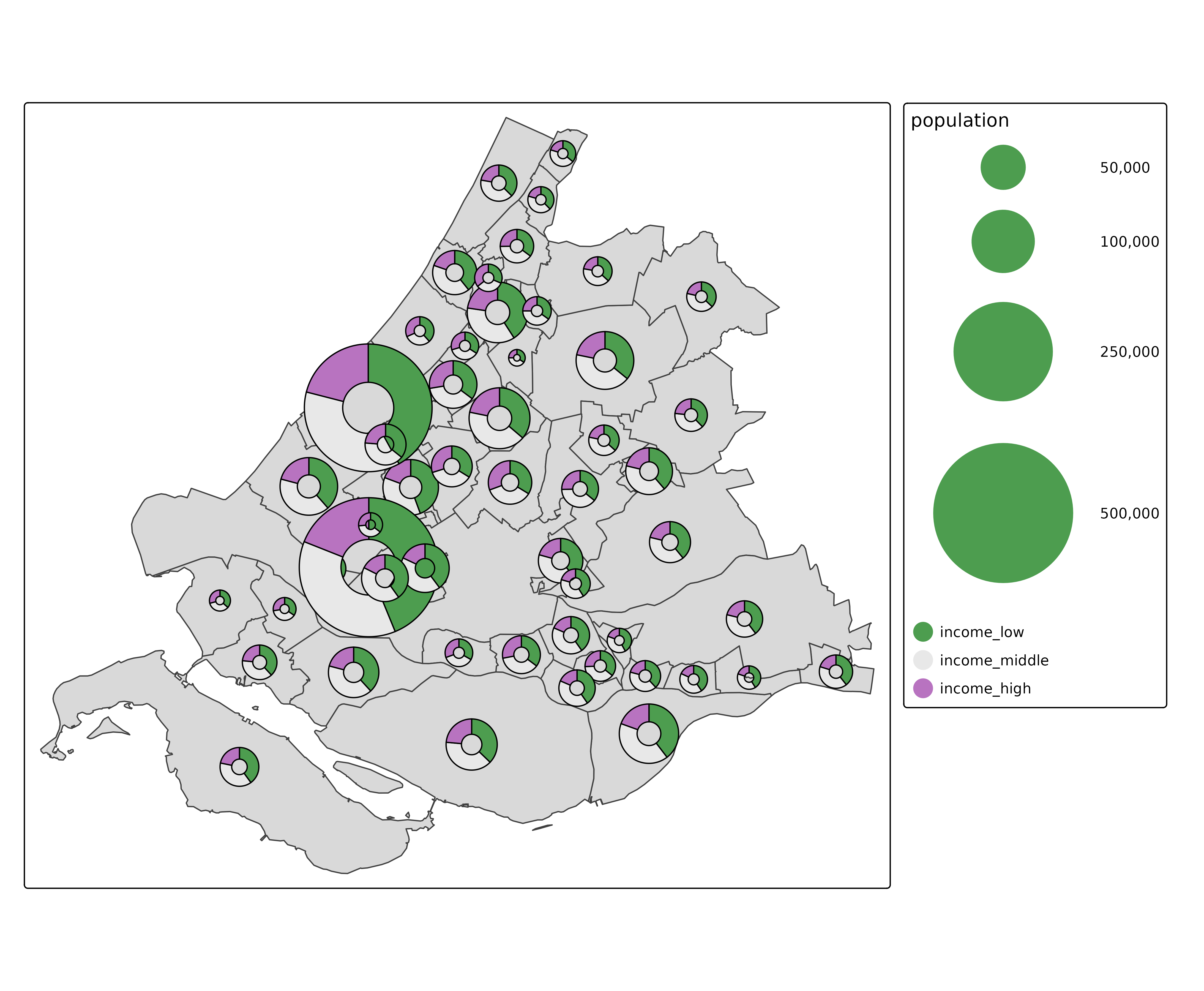
See tmap.glyphs.
A layer function tm_donuts is added. More glyph types layer
functions will follow, e.g. tm_pies, or
tm_radars.
library(tmap.glyphs)
ZH_muni = NLD_muni[NLD_muni$province == "Zuid-Holland", ]
ZH_muni$income_middle = 100 - ZH_muni$income_high - ZH_muni$income_low
tm_shape(ZH_muni) +
tm_polygons() +
tm_donuts(
parts = tm_vars(c("income_low", "income_middle", "income_high"), multivariate = TRUE),
fill.scale = tm_scale_categorical(values = "-pu_gn_div"),
size = "population",
size.scale = tm_scale_continuous(ticks = c(50000, 100000, 250000, 500000))) 
New spatial data classes
This type of extension requires methods to obtain:
- the spatial geometries (cast to either vectorized objects
(
sfc) or a stars object with indices) and - the data variables and its levels (if any)
See tmap.networks
which supports sfnetworks
library(sfnetworks)
library(tmap.networks)
(sfn = as_sfnetwork(roxel))
#> # A sfnetwork with 701 nodes and 851 edges
#> #
#> # CRS: EPSG:4326
#> #
#> # A directed multigraph with 14 components with spatially explicit edges
#> #
#> # Node data: 701 × 1 (active)
#> geometry
#> <POINT [°]>
#> 1 (7.533722 51.95556)
#> 2 (7.533461 51.95576)
#> 3 (7.532442 51.95422)
#> 4 (7.53209 51.95328)
#> 5 (7.532709 51.95209)
#> 6 (7.532869 51.95257)
#> # ℹ 695 more rows
#> #
#> # Edge data: 851 × 5
#> from to name type geometry
#> <int> <int> <chr> <fct> <LINESTRING [°]>
#> 1 1 2 Havixbecker Strasse residential (7.533722 51.95556, 7.533461 51…
#> 2 3 4 Pienersallee secondary (7.532442 51.95422, 7.53236 51.…
#> 3 5 6 Schulte-Bernd-Strasse residential (7.532709 51.95209, 7.532823 51…
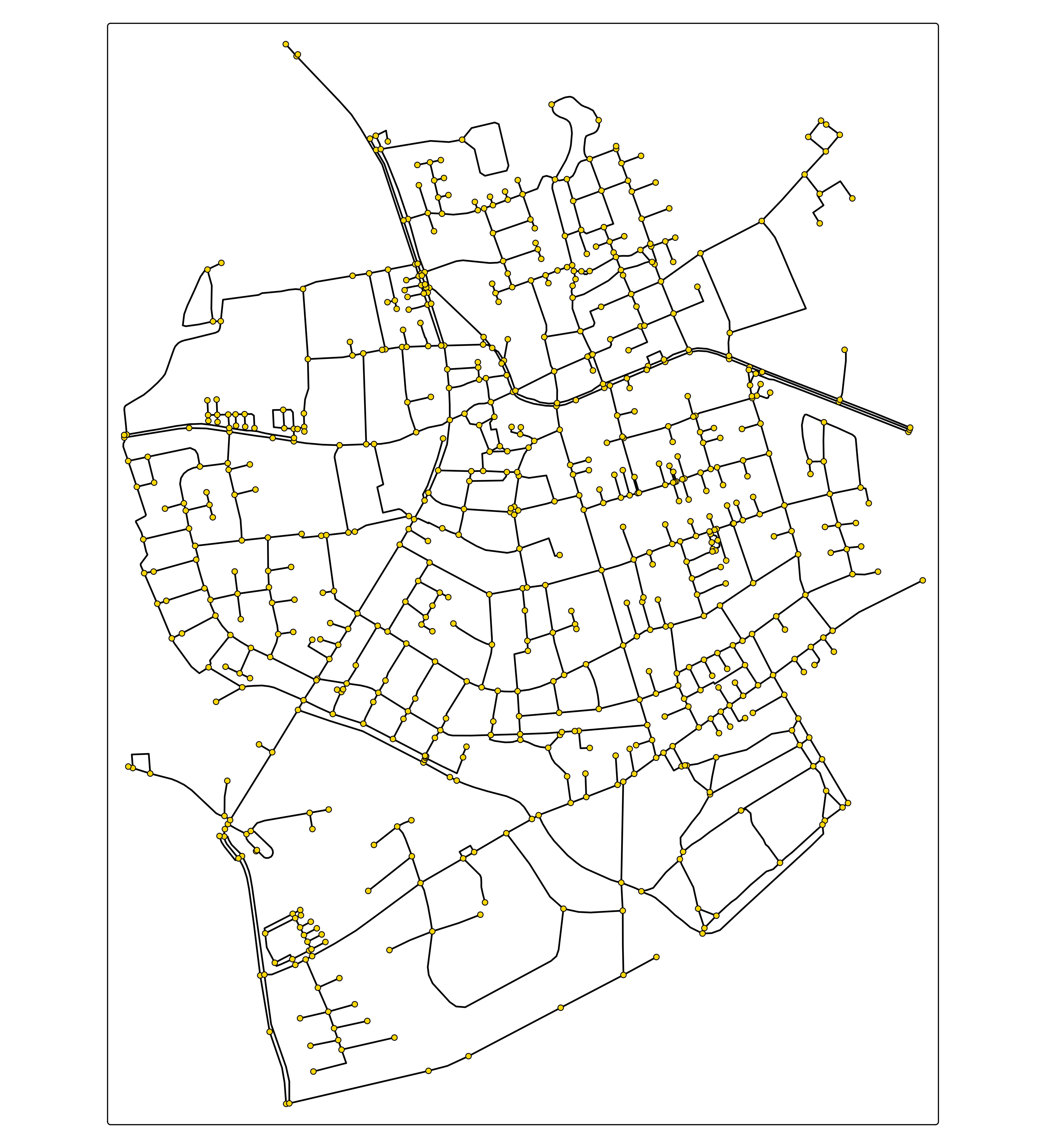
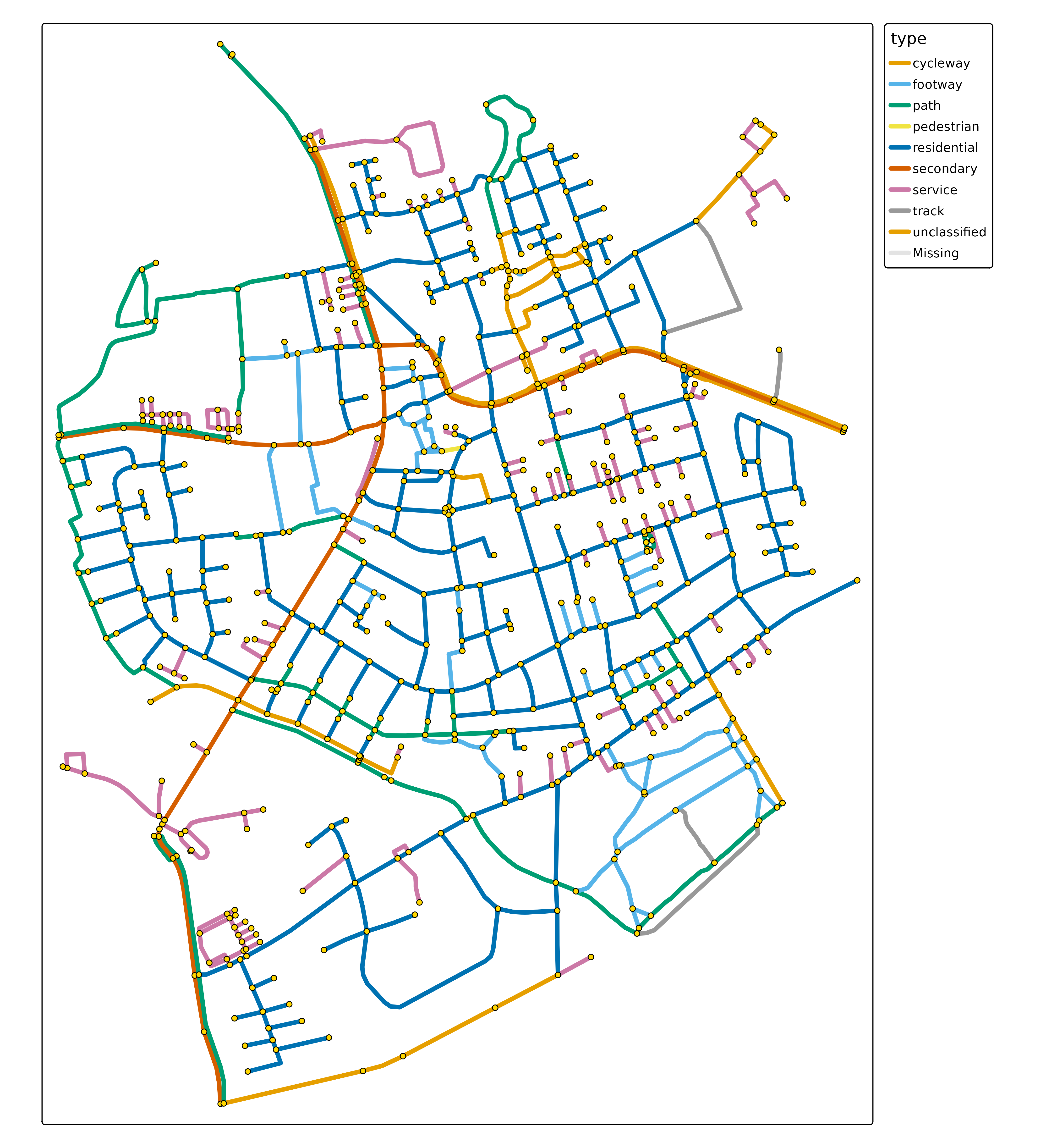
#> # ℹ 848 more rowsBesides this new spatial data class "sfnetwork", this
package also features new map layers, albeit very basic so far:
tm_shape(sfn) +
tm_network()

New mode
This type of extension is the most difficult one. It requires:
- Initialization
- Loading of the used spatial object
- Plotting function for each map layer type
- A function for each map component
- Functions to preprocess and show the legends
- Run the plot
- Shiny integration functions
A package in development tmap.mapgl
contains two new modes, "mapbox" and
"maplibre".
The shiny integration may not work yet.
tmap_mode("maplibre")
#> ℹ tmap modes "plot" -> "view" -> "mapbox" -> "maplibre"
#> ℹ rotate with `tmap::rtm()`switch to "plot" with `tmap::ttm()`
tm_shape(NLD_dist) +
tm_polygons(
fill = "employment_rate",
fill.scale = tm_scale_intervals(values = "scico.roma"),
lwd = 0.1) +
tm_shape(NLD_muni) +
tm_polygons(fill = NULL, lwd = 1) +
tm_maplibre(pitch = 70)