tmap basics: charts

Introduction

Each visual variable (e.g. fill in tm_polygons()) has an additional .chart argument via which charts can be shown:

tm_shape(World) +
  tm_polygons(
    fill = "press",
    fill.scale = tm_scale_intervals(n=10, values = "scico.hawaii"),
    fill.legend = tm_legend("World Press\nFreedom Index"),
    fill.chart = tm_chart_bar()) +
tm_crs("auto")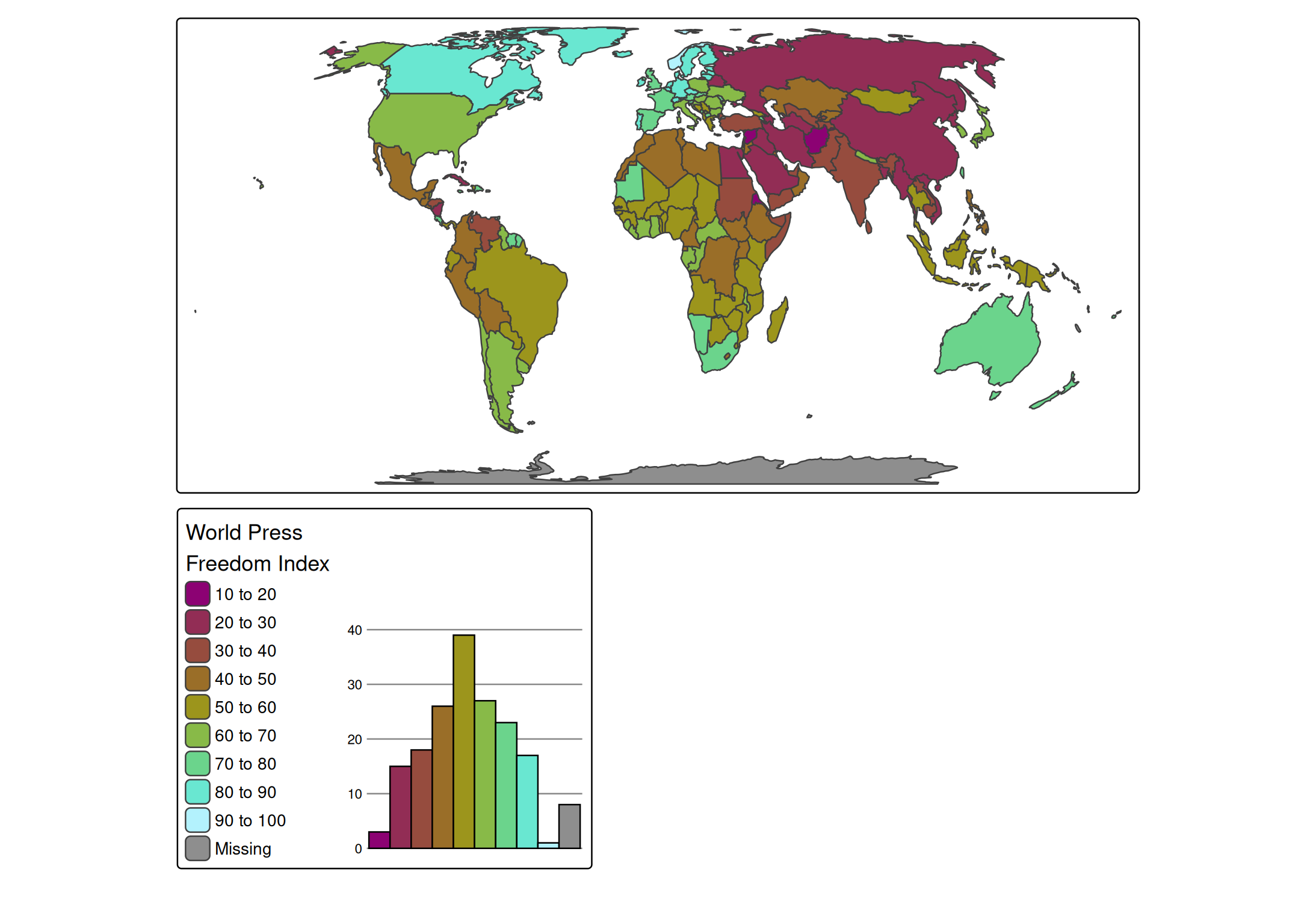

Chart types

Numeric variables

tm_shape(World) +
  tm_polygons("HPI",
    fill.scale = tm_scale_intervals(),
    fill.chart = tm_chart_donut())
#> [tip] Consider a suitable map projection, e.g. by adding `+ tm_crs("auto")`.
#> This message is displayed once per session.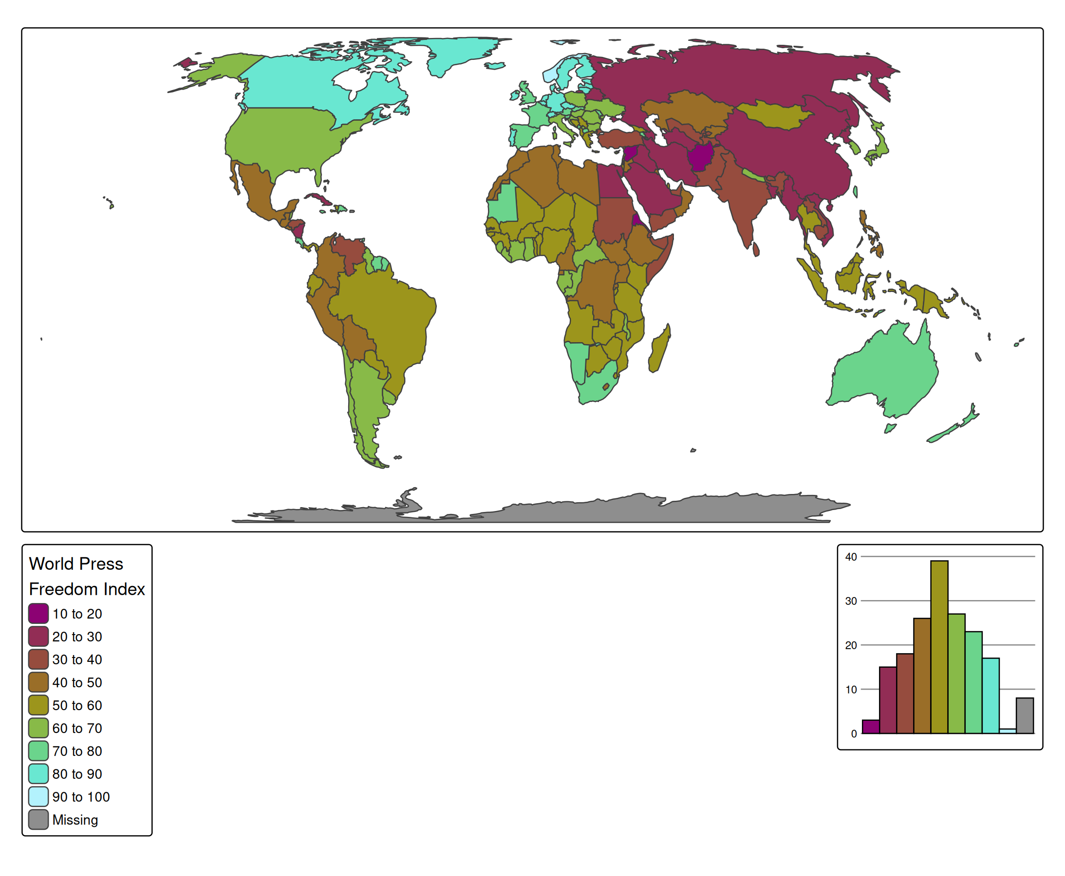

tm_shape(World) +
  tm_polygons("HPI",
    fill.scale = tm_scale_intervals(),
    fill.chart = tm_chart_box())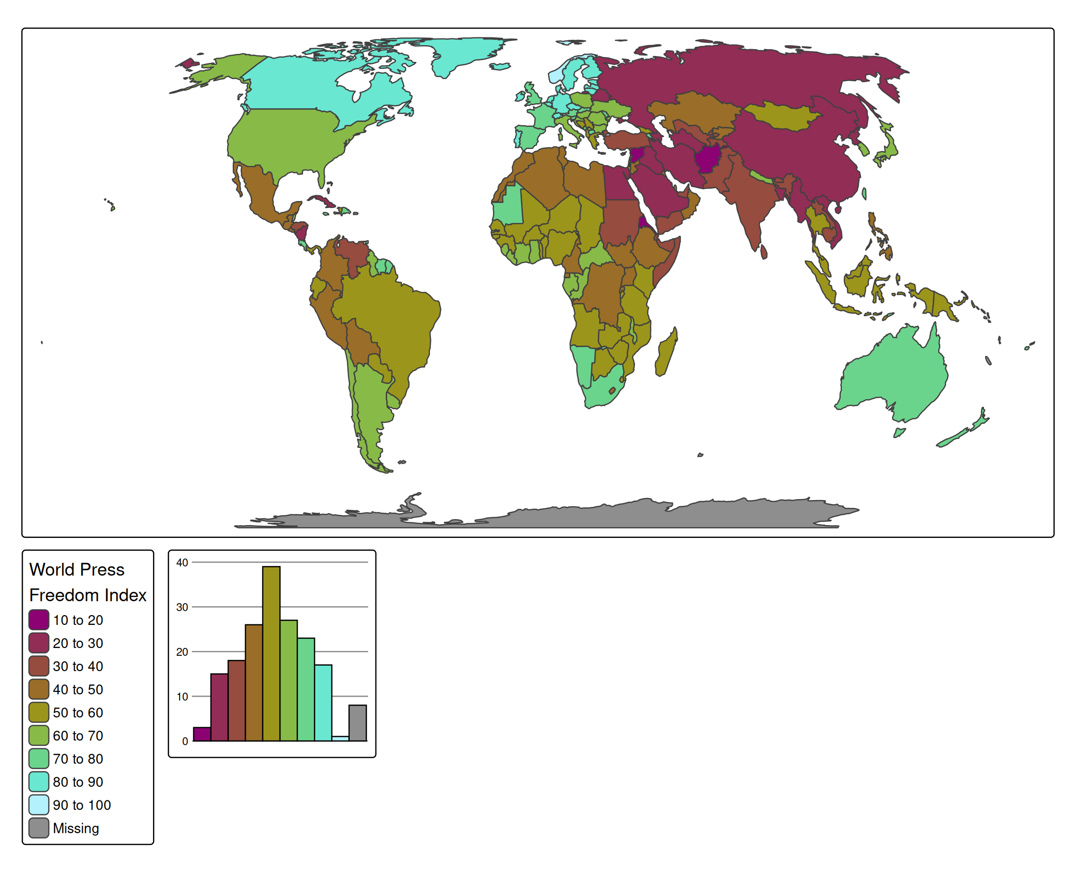

tm_shape(World) +
  tm_polygons("HPI",
    fill.scale = tm_scale_intervals(),
    fill.chart = tm_chart_violin())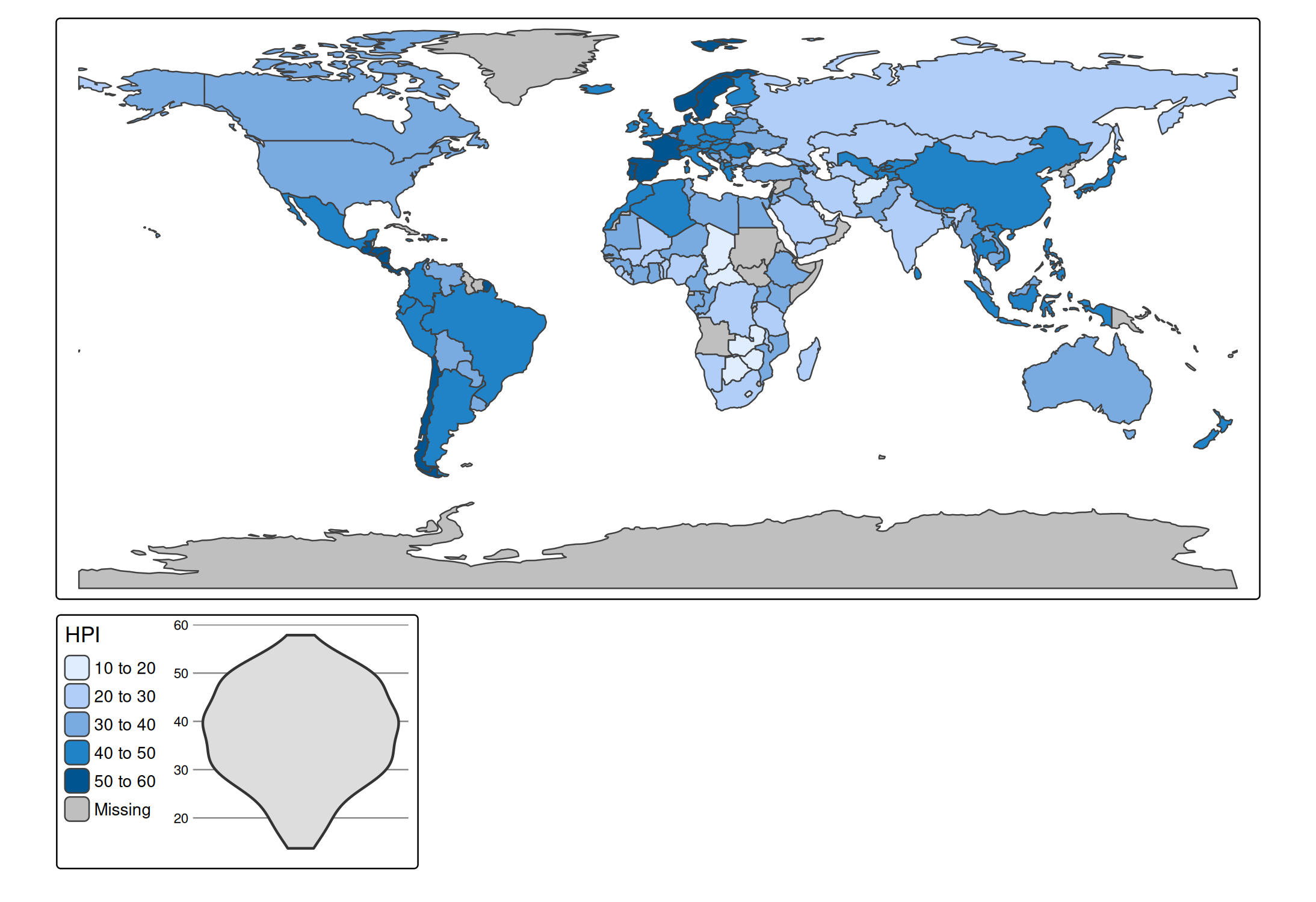

Categorical variable

tm_shape(World) +
  tm_polygons("economy",
    fill.scale = tm_scale_categorical(),
    fill.chart = tm_chart_bar())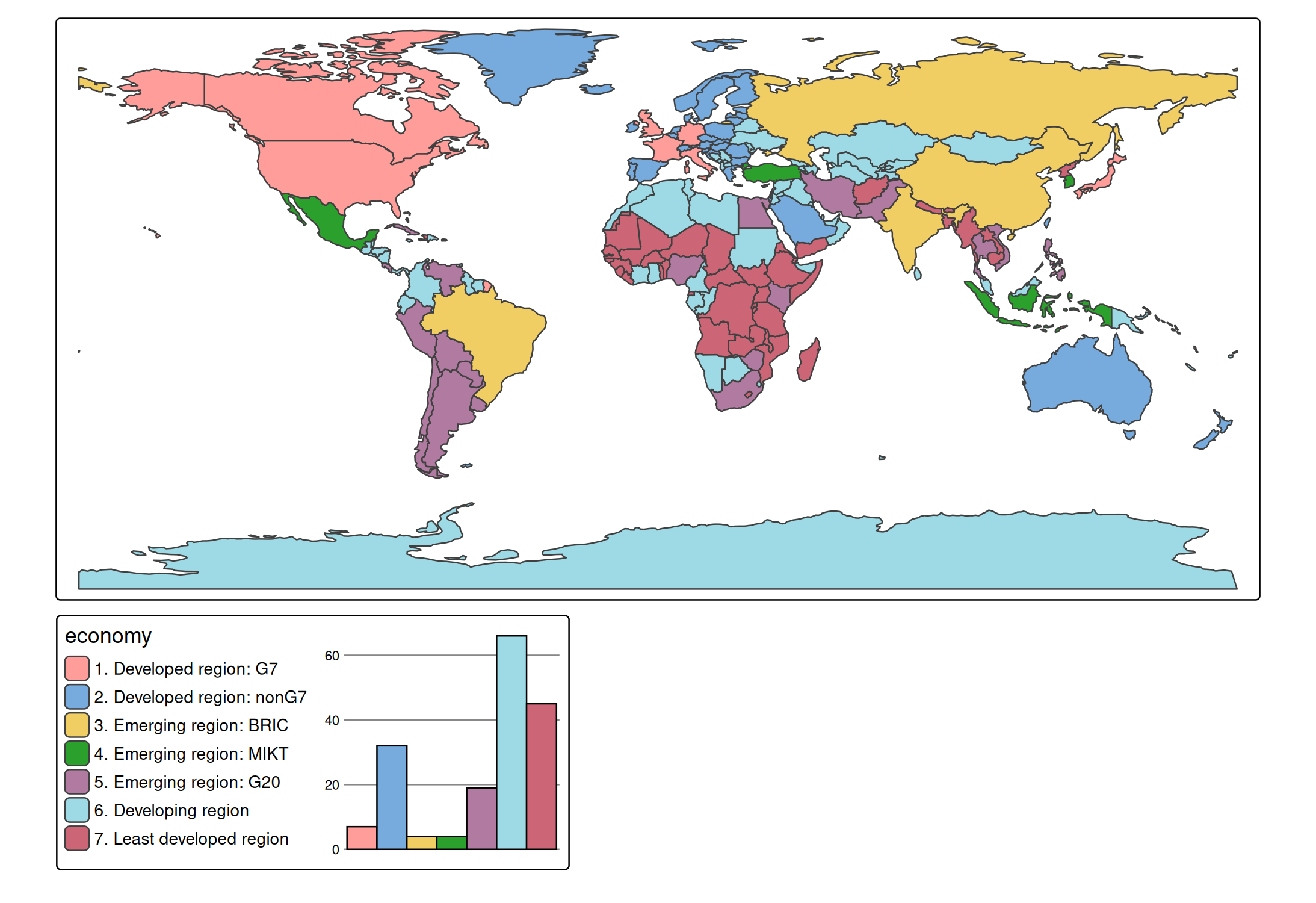

tm_shape(World) +
  tm_polygons("economy",
    fill.scale = tm_scale_categorical(),
    fill.chart = tm_chart_donut())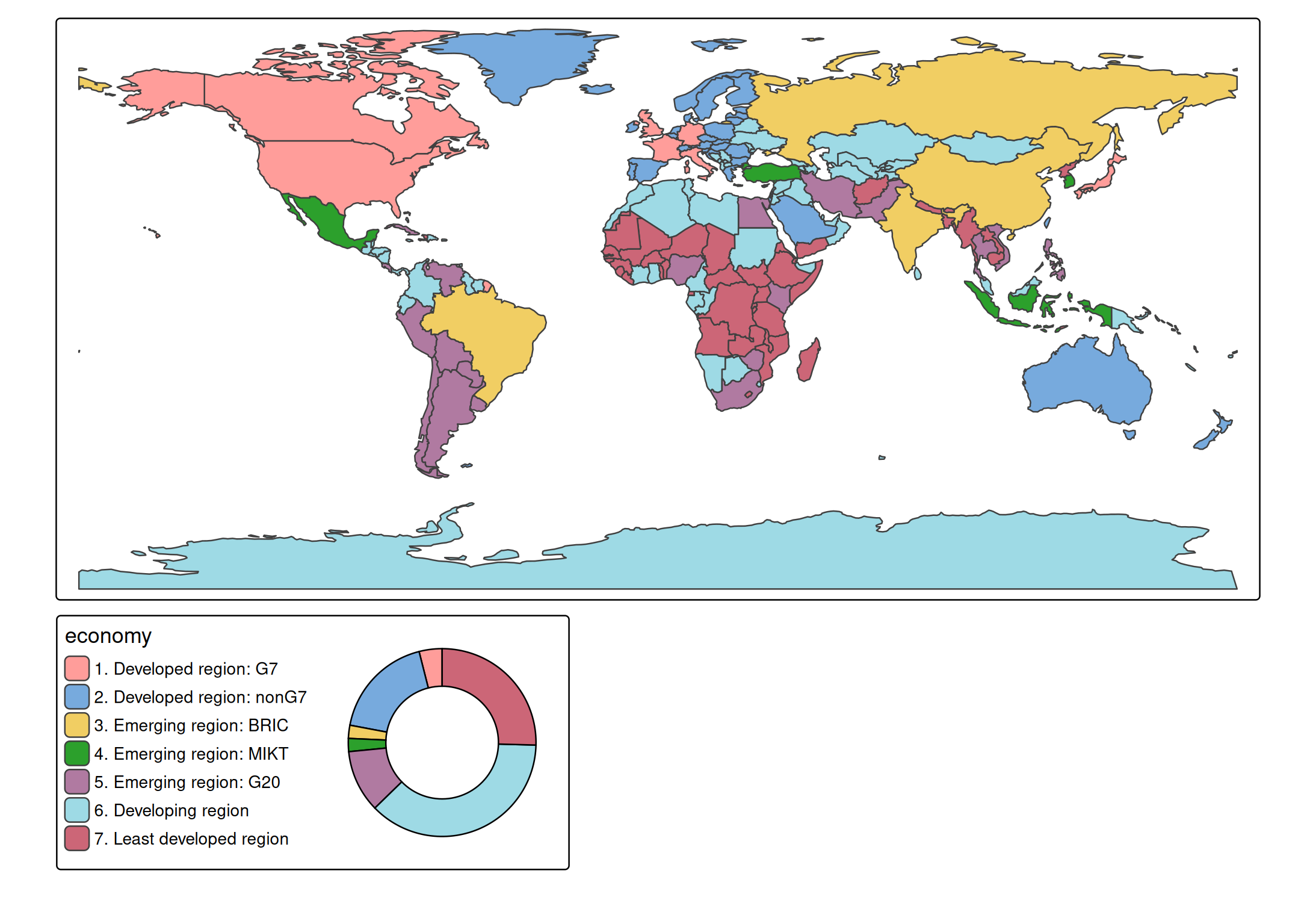

Bivariate charts

tm_shape(World) +
  tm_polygons(tm_vars(c("HPI", "well_being"), multivariate = TRUE),
    fill.chart = tm_chart_heatmap())
#> Labels abbreviated by the first letters, e.g.: "2 to 3" => "2"

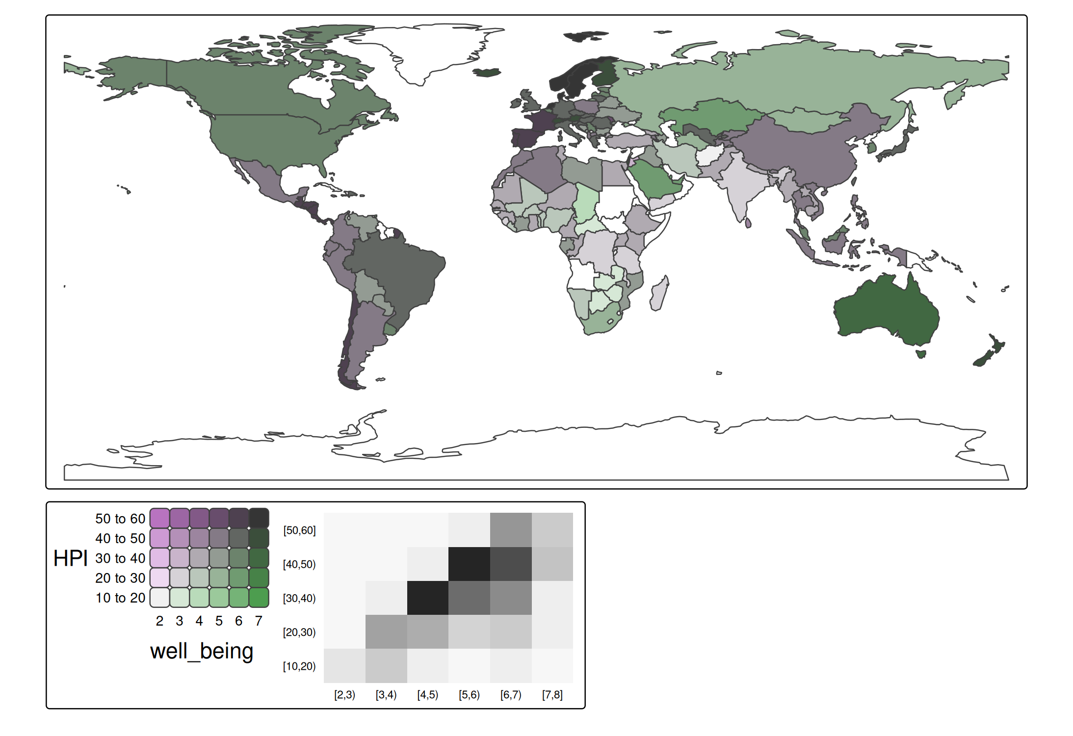
Position

We can update the position of the chart to bottom right (in a separate frame). See vignette about positioning.

tm_shape(World) +
  tm_polygons(
    fill = "press",
    fill.scale = tm_scale_intervals(n=10, values = "scico.hawaii"),
    fill.legend = tm_legend("World Press\nFreedom Index"),
    fill.chart = tm_chart_bar(position = tm_pos_out("center", "bottom", pos.h = "right"))) +
tm_crs("auto")

Or, in case we would like the chart to be next to the legend, but in a different frame:

tm_shape(World) +
  tm_polygons(
    fill = "press",
    fill.scale = tm_scale_intervals(n=10, values = "scico.hawaii"),
    fill.legend = tm_legend("World Press\nFreedom Index", group.frame = FALSE),
    fill.chart = tm_chart_bar(position = tm_pos_out("center", "bottom", align.v = "top"))) +
    tm_layout(component.stack_margin = .5) +
tm_crs("auto")

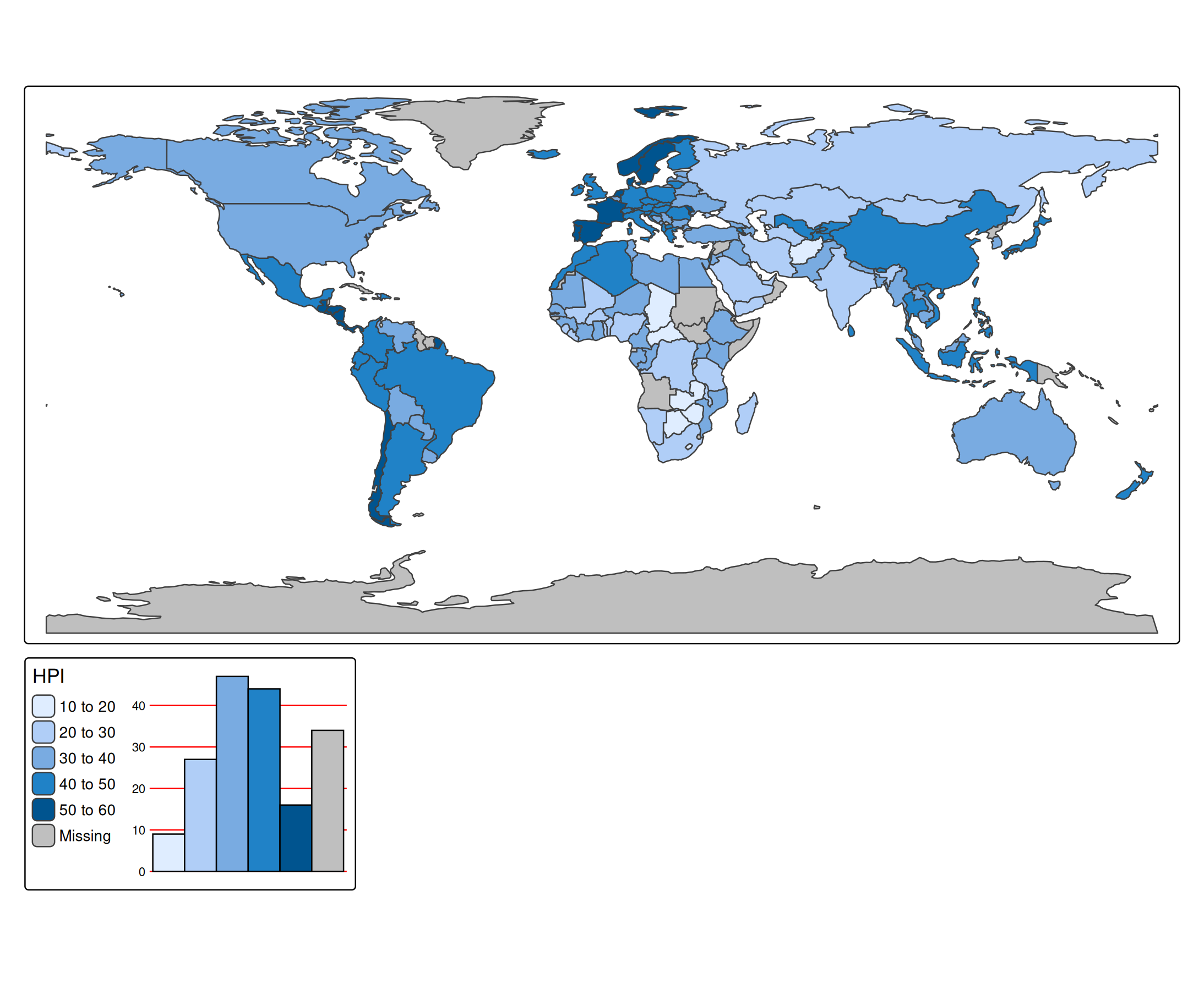
Additional ggplot2 code

require(ggplot2)
#> Loading required package: ggplot2
tm_shape(World) +
  tm_polygons("HPI",
    fill.scale = tm_scale_intervals(),
    fill.chart = tm_chart_bar(
      extra.ggplot2 = theme(
        panel.grid.major.y = element_line(colour = "red")
      ))
    )