tmap extensions: tmap.mapgl

There are two modes included in tmap: "plot" for static mapping and "view" for interactive mapping. See introduction. The "view" mode uses the JavaScript library Leaflet as backend.

The extension package tmap.mapgl offers two new modes which are also interactive: "mapbox" and "maplibre" which use the JavaScript libraries Mapbox GL and Maplibre GL respectively. The latter is a open source fork of the former before it went from open to closed source.

An API key is required to use "mapbox" (free for personal use, see instructions), but "maplibre" is (as the name suggests) free for any use.

Note that tmap.mapgl is a bridge between the R packages mapgl and tmap. It makes the functionality of mapgl (making the JavaScript libraries available to R) also available via the tmap user interface.

For this example we’ll create a choropleth of well being per country. We assign the map to map without showing it.

map = tm_shape(World) + 
  tm_polygons("well_being",
    fill.scale = tm_scale_continuous(values = "pu_gn"))

tmap_mode("plot")
#> ℹ tmap modes "plot" -> "view" -> "mapbox" -> "maplibre"
#> ℹ rotate with `tmap::rtm()`switch to "plot" with `tmap::ttm()`
map
#> [tip] Consider a suitable map projection, e.g. by adding `+ tm_crs("auto")`.
#> This message is displayed once per session.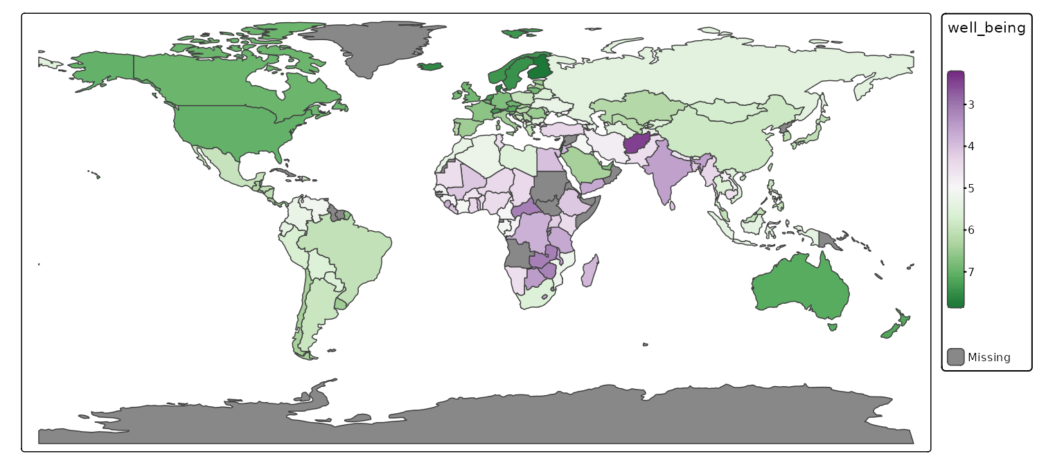

maplibre

library(tmap.mapgl)
tmap_mode("maplibre")
#> ℹ tmap modes "plot" -> "view" ->
#> "mapbox" -> "maplibre"
map

mapbox

For "mapbox" an API key is required, which is free for personal use. See instructions.

tmap_mode("mapbox")
map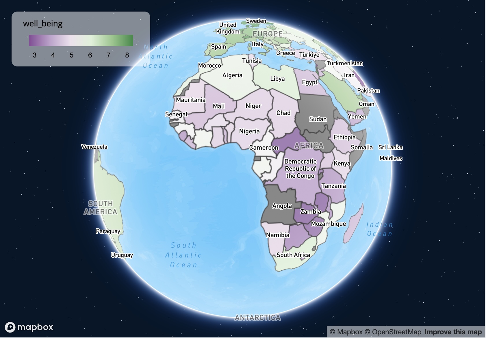

tmap mapbox mode

3d polygons

tmap.mapgl also features a new layer type, tm_polygons_3d, which is only available for "mapbox" and "maplibre".

This map layer is the same as tm_polygons, but one addition: polygons can be extruded in 3d shape. The visual variable to control this is called height.

Below an example of population density per country:

tmap_mode("maplibre")
#> ℹ tmap modes "plot" -> "view" ->
#> "mapbox" -> "maplibre"
tm_shape(World) +
    tm_polygons_3d(height = "pop_est_dens", fill = "continent")

Note that this is a toy simple example that does not take high population density of urban areas in otherwise sparse populated countries into account.

A more useful example of population density mapping is the following map of the Netherlands in which height is the population density per neighborhood (and therefore its volume represents population). Color is used to show the variable of interest, in this case education level.

tmap_mode("maplibre")
#> ℹ tmap modes "plot" -> "view" ->
#> "mapbox" -> "maplibre"

NLD_dist$pop_dens = NLD_dist$population / NLD_dist$area

tm_shape(NLD_dist) +
  tm_polygons_3d(height = "pop_dens",
    fill = "edu_appl_sci",
    fill.scale = tm_scale_intervals(style = "kmeans", values = "-pu_gn"),
    fill.legend = tm_legend("Univeristy degree")) +
tm_maplibre(pitch = 45)