Map layer: simple features

Map layer that draws simple features as they are. Supported visual variables are: fill (the fill color), col (the border color), size the point size, shape the symbol shape, lwd (line width), lty (line type), fill_alpha (fill color alpha transparency) and col_alpha (border color alpha transparency).

Usage

tm_sf(
  fill = tm_const(),
  fill.scale = tm_scale(),
  fill.legend = tm_legend(),
  fill.free = NA,
  col = tm_const(),
  col.scale = tm_scale(),
  col.legend = tm_legend(),
  col.free = NA,
  size = tm_const(),
  size.scale = tm_scale(),
  size.legend = tm_legend(),
  size.free = NA,
  shape = tm_const(),
  shape.scale = tm_scale(),
  shape.legend = tm_legend(),
  shape.free = NA,
  lwd = tm_const(),
  lwd.scale = tm_scale(),
  lwd.legend = tm_legend(),
  lwd.free = NA,
  lty = tm_const(),
  lty.scale = tm_scale(),
  lty.legend = tm_legend(),
  lty.free = NA,
  fill_alpha = tm_const(),
  fill_alpha.scale = tm_scale(),
  fill_alpha.legend = tm_legend(),
  fill_alpha.free = NA,
  col_alpha = tm_const(),
  col_alpha.scale = tm_scale(),
  col_alpha.legend = tm_legend(),
  col_alpha.free = NA,
  linejoin = "round",
  lineend = "round",
  plot.order.list = list(polygons = tm_plot_order("AREA"), lines =
    tm_plot_order("LENGTH"), points = tm_plot_order("size")),
  options = opt_tm_sf(),
  zindex = NA,
  group = NA,
  group.control = "check",
  blend = "over",
  ...
)

opt_tm_sf(
  polygons.only = "yes",
  lines.only = "yes",
  points_only = "yes",
  point_per = "feature",
  points.icon.scale = 3,
  points.just = NA,
  points.grob.dim = c(width = 48, height = 48, render.width = 256, render.height = 256)
)

Arguments

fill, fill.scale, fill.legend, fill.free: Visual variable that determines the fill color. See details. Unit: Color – a color name, hex string.
col, col.scale, col.legend, col.free: Visual variable that determines the color. See details. Unit: Color – a color name, hex string.
size, size.scale, size.legend, size.free: Visual variable that determines the size. See details. Unit: Typographic lines ("lines"); 1 line is approx. 1/6 inch. Controlled by values.scale and tmap_options(values.scale = ...).
shape, shape.scale, shape.legend, shape.free: Visual variable that determines the shape. See details. Unit: Integer pch code (1-25) used as a plotting symbol. See example of tm_symbols()
lwd, lwd.scale, lwd.legend, lwd.free: Visual variable that determines the line width. See details. Unit: Base R line-width units; 1 lwd is approx. 0.75 pt at 96 dpi.
lty, lty.scale, lty.legend, lty.free: Visual variable that determines the line type. See details. Unit: Integer (1-6) or name: "solid", "dashed", "dotted", "dotdash", "longdash", "twodash".
fill_alpha, fill_alpha.scale, fill_alpha.legend, fill_alpha.free: Visual variable that determines the fill color transparency. See details. Unit: Proportion – numeric 0-1 (0 = fully transparent, 1 = fully opaque).
col_alpha, col_alpha.scale, col_alpha.legend, col_alpha.free: Visual variable that determines the color transparency. See details. Unit: Proportion – numeric 0-1 (0 = fully transparent, 1 = fully opaque).
linejoin, lineend: line join and line end. See gpar() for details.
plot.order.list: Specification in which order the spatial features are drawn. This consists of a list of three elementary geometry types: for polygons, lines and, points. For each of these types, which are drawn in that order, a tm_plot_order() is required.
options: options passed on to the corresponding opt_<layer_function> function
zindex: Controls the stacking order of map layers. Should be set to a value above 400. By default, layers are stacked in call order, starting at 401. See details.
group: Name of the group to which this layer belongs. This is only relevant in view mode, where layer groups can be switched (see group.control)
group.control: In view mode, the group control determines how layer groups can be switched on and off. Options: "radio" for radio buttons (meaning only one group can be shown), "check" for check boxes (so multiple groups can be shown), and "none" for no control (the group cannot be (de)selected).
blend: Compositing operator for layer blending, applied to each sublayer (polygons, lines, points). Default "over" applies no blending. See the "Layer blending" section of tm_polygons() for supported values.
...: passed on to tm_polygons(), tm_lines(), and tm_dots()
polygons.only: should only polygon geometries of the shape object (defined in tm_shape()) be plotted? By default "ifany", which means TRUE in case a geometry collection is specified.
lines.only: should only line geometries of the shape object (defined in tm_shape()) be plotted, or also other geometry types (like polygons)? By default "ifany", which means TRUE in case a geometry collection is specified.
points_only: should only point geometries of the shape object (defined in tm_shape()) be plotted? By default "ifany", which means TRUE in case a geometry collection is specified.
point_per: specification of how spatial points are mapped when the geometry is a multi line or a multi polygon. One of "feature", "segment" or "largest". The first generates a spatial point for every feature, the second for every segment (i.e. subfeature), the third only for the largest segment (subfeature). Note that the last two options can be significant slower.
points.icon.scale: scaling number that determines how large the icons (or grobs) are in plot mode in comparison to proportional symbols (such as bubbles). For view mode, use the argument grob.dim
points.just: justification of the points relative to the point coordinates. Either one of the following values: "left" , "right", "center", "bottom", and "top", or a vector of two values where first value specifies horizontal and the second value vertical justification. Besides the mentioned values, also numeric values between 0 and 1 can be used. 0 means left justification for the first value and bottom justification for the second value. Note that in view mode, only one value is used.
points.grob.dim: vector of four values that determine how grob objects (see details) are shown in view mode. The first and second value are the width and height of the displayed icon. The third and fourth value are the width and height of the rendered png image that is used for the icon. Generally, the third and fourth value should be large enough to render a ggplot2 graphic successfully. Only needed for the view mode.

Details

The visual variable arguments (e.g. col) can be specified with a data variable name (e.g., a spatial vector attribute or a raster layer of the object specified in tm_shape()), with a visual value (for col, a color is expected), or with a geometry-derived variable (see below). See vignette: Visual variables.

Multiple values can be specified: in that case facets are created. These facets can be combined with other faceting data variables, specified with tm_facets(). See vignette: Facets.

The *.scale arguments determine the used scale to map the data values to visual variable values. These can be specified with one of the available tm_scale_*() functions. The default is specified by the tmap option (tm_options()) scales.var. See `rvignette: Scales
The *.legend arguments determine the used legend, specified with tm_legend(). The default legend and its settings are determined by the tmap options (tm_options()) legend. . See `rvignette: Legends
The *.chart arguments specify additional charts, specified with tm_chart_, e.g. tm_chart_histogram(). See `rvignette: Charts
The *.free arguments determine whether scales are applied freely across facets, or shared. A logical value is required. They can also be specified with a vector of three logical values; these determine whether scales are applied freely per facet dimension. This is only useful when facets are applied (see tm_facets()). There are maximally three facet dimensions: rows, columns, and pages. This only applies for a facet grid (tm_facets_grid()). For instance, col.free = c(TRUE, FALSE, FALSE) means that for the visual variable col, each row of facets will have its own scale, and therefore its own legend. For facet wraps and stacks (tm_facets_wrap() and tm_facets_stack()) there is only one facet dimension, so the *.free argument requires only one logical value.

Currently, three geometry-derived variables are implemented:

"AREA" (polygons only), which uses the feature area;
"LENGTH" (lines only), which uses the feature length; and
"MAP_COLORS", which assigns values so that adjacent features receive different values, making it particularly suitable for coloring neighbouring polygons.

Note that geometry-derived variables do not generate a legend automatically. If a legend is required, compute the corresponding variable explicitly, for example with sf::st_area(), sf::st_length(), or tmaptools::map_coloring(), and use the resulting values instead.

Visual variable units

Every visual variable maps data values to a specific output unit. Knowing the unit matters when supplying constant values via tm_const(), or output ranges via values.range / values.scale in the scale functions.

Variable	Output unit	Notes
`fill`, `col`, `bgcol`	color	name, hex, or palette string
`fill_alpha`, `col_alpha`, `bgcol_alpha`	proportion 0-1	0 = transparent, 1 = opaque
`size` (symbols, bubbles, squares, dots)	typographic lines	1 line approx. 1/6 inch; scaled by `values.scale`
`size` (circles)	meters	plain numeric or a `units` object
`size` (text, labels)	multiplier	1 = 12 pt (plot) / 12 px (view)
`lwd`	lwd	base R units; 1 lwd approx. 0.75 pt at 96 dpi
`lty`	–	integer 1-6 or name ("solid", "dashed", ...)
`shape`	–	integer `pch` 1-25 or single character
`angle`	degrees	0-360, clockwise from north
`fontface`	–	"plain", "bold", "italic", "bold.italic"

Symbol size (`size` in `tm_symbols`, `tm_bubbles`, `tm_squares`, `tm_dots`)

"Lines" is a typographic unit: one line is approximately 1/6 inch (the default base line-height in R graphics). The global multiplier tmap_options(values.scale = list(size.bubbles = 1.5)) scales all symbol sizes without changing the data mapping.

Circle size (`size` in `tm_circles`)

The value is a geographic radius in meters. A plain numeric vector is interpreted as meters; a units object (from the units package) is automatically converted, so units::as_units(1, "mi") gives a 1-mile radius. Because the radius is geographic, circles scale with zoom in interactive (view) mode – unlike bubble symbols which keep a fixed screen size.

Text size (`size` in `tm_text`, `tm_labels`)

The value is a multiplier of the base font size. size = 1 renders at 12 pt in plot mode (R's default par("ps")) and at 12 px in view mode (gp$cex * 12 px, see tmapLeafletDataPlot.tm_data_text); the two modes are consistent by design.

Layer blending (`blend`)

Blend modes control how a layer's pixels are combined with the pixels beneath it. For each pixel, let $S$ be the source (top layer) RGB value and $D$ be the destination (bottom layer) RGB value, both normalised to $[0, 1]$.

`blend`	Formula	Use case
`"over"`	$S \cdot \alpha + D \cdot (1 - \alpha)$	Standard alpha compositing (default)
`"multiply"`	$S \times D$	Hillshading over colour raster; both layers darken each other
`"screen"`	$1 - (1 - S)(1 - D)$	Inverse of multiply; brightens
`"overlay"`	multiply if $D < 0.5$, screen if $D \geq 0.5$	Boosts contrast; preserves midtones
`"darken"`	$\min(S, D)$	Keeps the darker of the two layers per channel
`"lighten"`	$\max(S, D)$	Keeps the lighter of the two layers per channel

Requires R >= 4.2 and a compatible graphics device (e.g. png(type = "cairo"), svg()). In view mode, blending is applied via CSS mix-blend-mode. See grid::groupGrob() for the full list of supported operators.

zindex and pane names

In view mode, each layer is rendered in a Leaflet pane named "tmap{zindex}" (e.g., "tmap401", "tmap402"), with base tile layers placed in the standard "tile" pane.

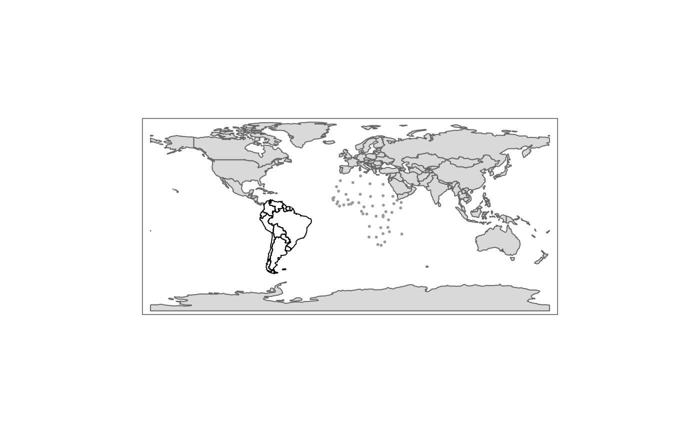
Examples

data(World)

World$geometry[World$continent == "Africa"] <- 
  sf::st_centroid(World$geometry[World$continent == "Africa"])
World$geometry[World$continent == "South America"] <- 
  sf::st_cast(World$geometry[World$continent == "South America"], 
    "MULTILINESTRING", group_or_split = FALSE)

tm_shape(World, crs = "+proj=robin") + 
  tm_sf()