library(tmap)
tmap_options(scale = 0.75)
In a dot density map, each dot represents a number of units, for
instance inhabitants. Dense areas get many dots, sparse areas few. This
example shows the population of the Netherlands for each of its 3340
districts (NLD_dist), first with one color, and then
colored by income class.
Dot density maps are made with a dot pattern (see the vignette
about fill patterns): the map variable pattern_density
determines the number of dots per area. With the scale
tm_scale_continuous_area(), the number of dots is
proportional to the data, so each dot represents the same number of
inhabitants.
Population density
The population density (inhabitants per km2) has the units 1/km2, since the area of the districts is in km2:
NLD = NLD_dist
NLD$pop_dens = NLD$population / NLD$area
summary(NLD$pop_dens)
#>    Min. 1st Qu.  Median    Mean 3rd Qu.    Max.
#>     0.0    96.9   375.6  1969.1  3083.2 28672.4
At the scale of the whole country, the dots should be small and close
together: otherwise, most districts are smaller than the area of one
dot, and each dot would represent many inhabitants. Therefore, the
density ranges from 0 to 5 (values = c(0, 5)) instead of
from 0 to 1, and the dots are small (pattern_size = 0.5).
The size of the dots does not change the number of inhabitants per dot,
which only depends on the density; in the densest areas, the dots merge.
The few districts with more than 10,000 inhabitants per km2
get the densest pattern (outliers.trunc). Instead of the
district borders, the province borders are drawn:
dens_scale = tm_scale_continuous_area(
  limits = c(0, 10000),
  values = c(0, 5),
  outliers.trunc = c(FALSE, TRUE),
  ticks = c(1000, 5000, 10000))

tm_shape(NLD) +
  tm_polygons(fill = "white", col = NULL,
              pattern = "stipple", pattern_size = 0.5, pattern_col = "grey10",
              pattern_density = "pop_dens",
              pattern_density.scale = dens_scale,
              pattern_density.legend = tm_legend(
                "Inhabitants per km2",
                dot.value = "1 dot ≈ {n} inhabitants")) +
tm_shape(NLD_prov) +
  tm_borders(col = "grey50", lwd = 0.8)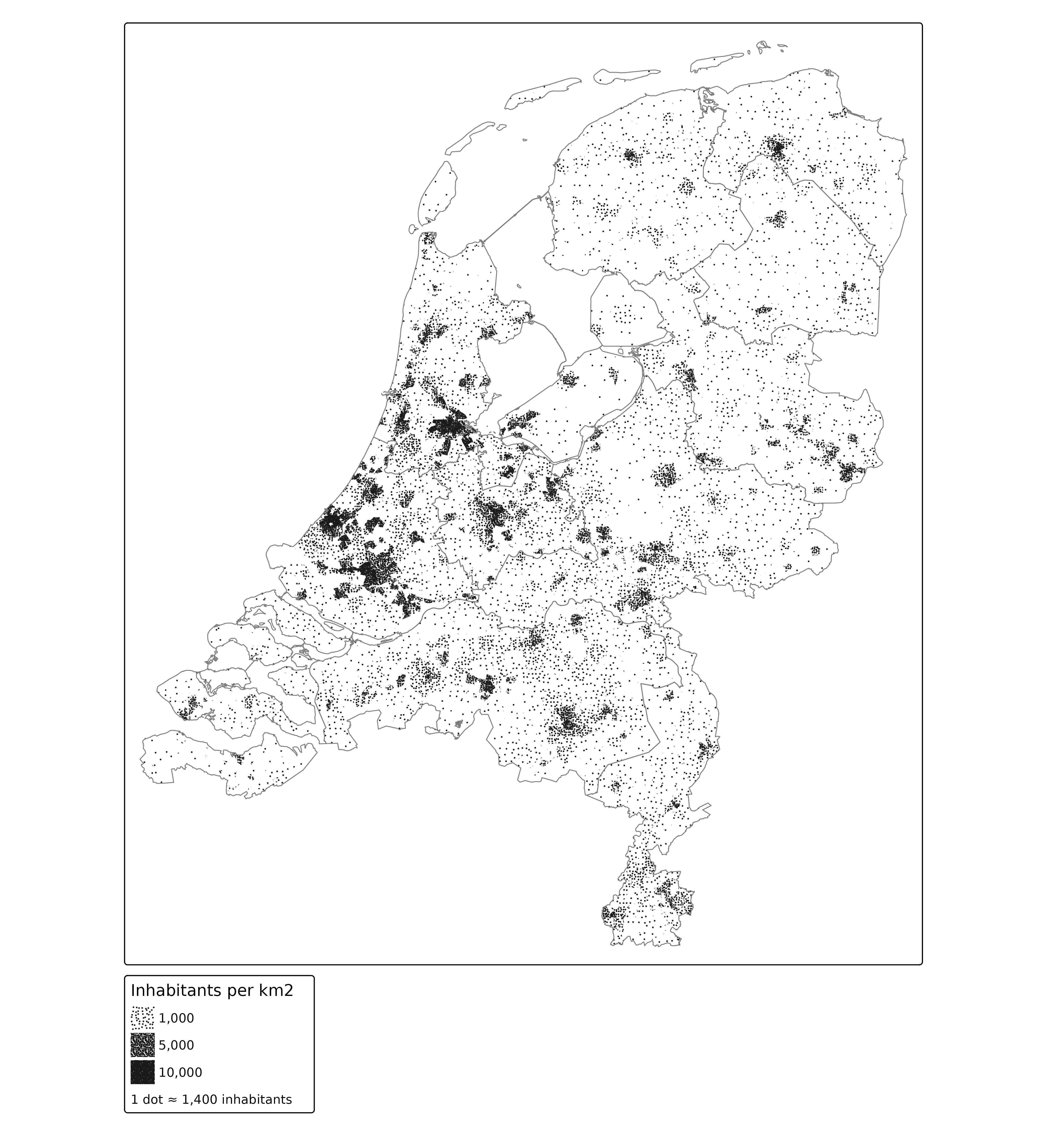
The number of inhabitants per dot depends on the map scale, and is
computed when the map is drawn (legend argument dot.value).
The dots are spread over each district; they do not show where people
live within a district. A district that is smaller than the area of one
dot gets either one dot or none, so the number of dots is only correct
on average.
Interactive version
In view mode, the number of inhabitants per dot is updated after zooming. To keep the map light, the district polygons are simplified (which is hardly visible at this scale), popups are disabled, and the district names are shown when hovering:
NLD_simple = sf::st_simplify(NLD, preserveTopology = TRUE, dTolerance = 100)

tmap_mode("view")
tm_shape(NLD_simple) +
  tm_polygons(fill = "white", col = NULL,
              popup = FALSE, id = "name",
              pattern = "stipple", pattern_size = 0.5, pattern_col = "grey10",
              pattern_density = "pop_dens",
              pattern_density.scale = dens_scale,
              pattern_density.legend = tm_legend(
                "Inhabitants per km2",
                dot.value = "1 dot \u2248 {n} inhabitants")) +
tm_shape(NLD_prov) +
  tm_borders(col = "grey50", lwd = 1.5)
tmap_mode("plot")In view mode, the dots keep their size and spacing on the screen when
zooming in, so zooming in shows more dots, each representing fewer
inhabitants. With opt_tm_polygons(pattern.zoom = TRUE), the
dots stick to the map instead, and each dot keeps representing the same
number of inhabitants.
Income classes
The data contain the percentage of individuals with a low income (the lowest 40% nationwide) and a high income (the highest 20% nationwide). The remaining percentage has a middle income. The population density of each class is the population density times this percentage:
NLD$income_middle = 100 - NLD$income_low - NLD$income_high
NLD$dens_low = NLD$pop_dens * NLD$income_low / 100
NLD$dens_middle = NLD$pop_dens * NLD$income_middle / 100
NLD$dens_high = NLD$pop_dens * NLD$income_high / 100
A polygon can have only one pattern, so each class is drawn as a
separate layer, with its own dot color. To make each dot represent the
same number of inhabitants in all three layers, the same scale is used
for each layer. The dots of the three layers would be placed at the same
positions in a district where two classes have the same density.
Therefore, each layer uses a different seed for the random
placement of the dots (see tm_patterns()).
The dots are slightly larger than in the map above
(pattern_size = 0.7), so that their colors can be
distinguished. The legends of the three layers would only differ in
color. Instead, the first one is shown in gray (the legend argument
pattern_col), and the colors are explained in a manual
legend (tm_add_legend()):
cols = c(low = "#D95F02", middle = "#1B9E77", high = "#7570B3")

dot_layer = function(var, col, seed, legend = tm_legend_hide(), fill = NULL) {
  tm_polygons(fill = fill, col = NULL,
              pattern = tm_patterns("stipple", seed = seed),
              pattern_size = 0.7, pattern_col = col,
              pattern_density = var,
              pattern_density.scale = dens_scale,
              pattern_density.legend = legend)
}

tm_shape(NLD) +
  dot_layer("dens_low", cols["low"], seed = 1, fill = "white",
            legend = tm_legend("Inhabitants per km2",
                               dot.value = "1 dot ≈ {n} inhabitants",
                               pattern_col = "grey20")) +
  dot_layer("dens_middle", cols["middle"], seed = 2) +
  dot_layer("dens_high", cols["high"], seed = 3) +
  tm_add_legend(type = "symbols", title = "Income",
                labels = c("Low (lowest 40%)", "Middle", "High (highest 20%)"),
                fill = cols, col = NA, size = 0.5) +
tm_shape(NLD_prov) +
  tm_borders(col = "grey50", lwd = 0.8)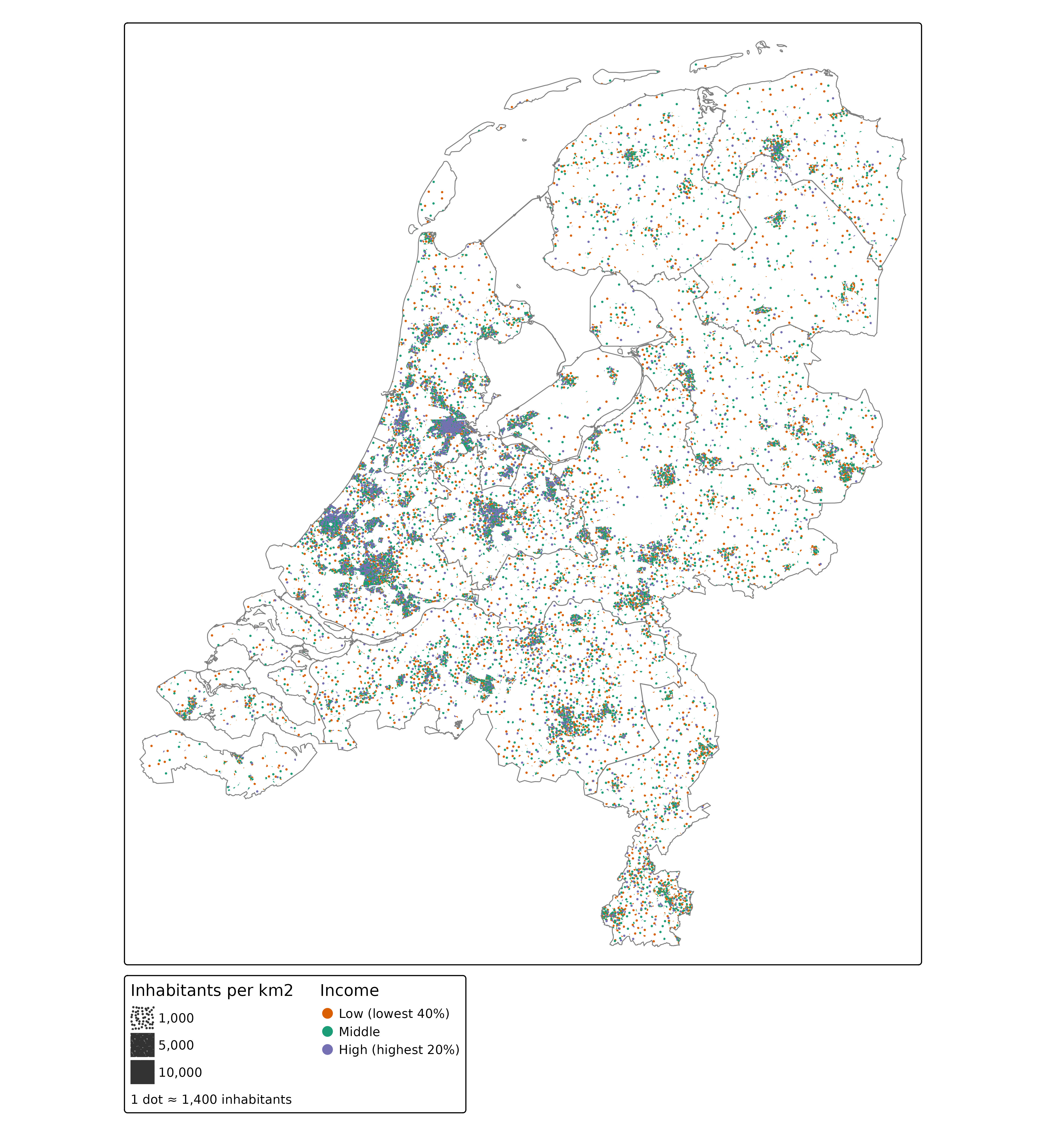
The share of high incomes is largest in the provinces Utrecht, Noord-Holland, and Zuid-Holland, especially around Amsterdam, Utrecht, and The Hague, whereas the share of low incomes is largest in the north (Groningen and Friesland). For 196 districts with few inhabitants, the income data are missing, so no dots are drawn there.
Note that the order of the layers matters: dots of later layers are drawn on top of dots of earlier layers. Since the dots are small and spread randomly, few dots overlap.